Equation of a Line, 3D Plane, and Hyperplane
1. Introduction
Imagine you’re standing at the edge of a football field, and you want to describe to a friend on the phone exactly where the halfway line is. You could say “it’s the line where, no matter how far left or right you walk, you’re always the exact same distance from either goal.” That’s basically what a line (or, in higher dimensions, a plane or hyperplane) does mathematically — it’s a boundary that splits a space into two neat halves based on a simple rule.
This idea might feel like basic 10th-grade geometry (you’ve probably drawn a hundred times), but it turns out to be one of the most important building blocks in machine learning. Algorithms like logistic regression and support vector machines (SVM) are, underneath all the jargon, just trying to find the best possible line/plane/hyperplane that separates one group of data points from another. Before you can understand how those algorithms “draw the boundary,” you need to be completely comfortable with what that boundary actually is, mathematically.
So in these notes, we’ll go on a journey: starting from the simple straight line you know from school, generalizing it to 3D (a plane), and then generalizing it further to any number of dimensions (a hyperplane) — the exact same idea used inside real ML models.
2. History
The story of the “equation of a line” doesn’t start with algebra — it starts with geometry. The Ancient Greeks, especially Euclid (around 300 BCE), described lines purely through shapes and relationships (postulates and axioms), with no coordinates or algebra involved at all. A line, to Euclid, was just “the shortest distance between two points” — a visual, geometric idea.
The turning point came almost 2000 years later with René Descartes in the 17th century. Descartes had the (now famous) insight of laying a grid of numbers — an x-axis and a y-axis — over geometric space. This is called the Cartesian coordinate system, named after him. Suddenly, a line wasn’t just a picture anymore — it was a set of coordinate pairs that satisfied an equation. This single idea merged two separate branches of math — geometry and algebra — into what we now call analytic geometry. It’s the reason you can write at all.
Once lines could be written as equations, mathematicians naturally asked: “What happens if we add a third axis, ?” That gave rise to describing planes in 3D space using very similar linear equations. And once linear algebra matured in the 19th and 20th centuries (with mathematicians like Cayley and Grassmann developing vector spaces and matrix notation), the idea generalized even further — to spaces with 4, 10, or 1000 dimensions, where the flat “boundary” is called a hyperplane. This generalization turned out to be exactly the tool needed a century later when computer scientists started building algorithms that separate data — and that’s why this “old” topic sits at the heart of modern machine learning today.
3. Core Concepts
3.1 The Straight Line (2D)
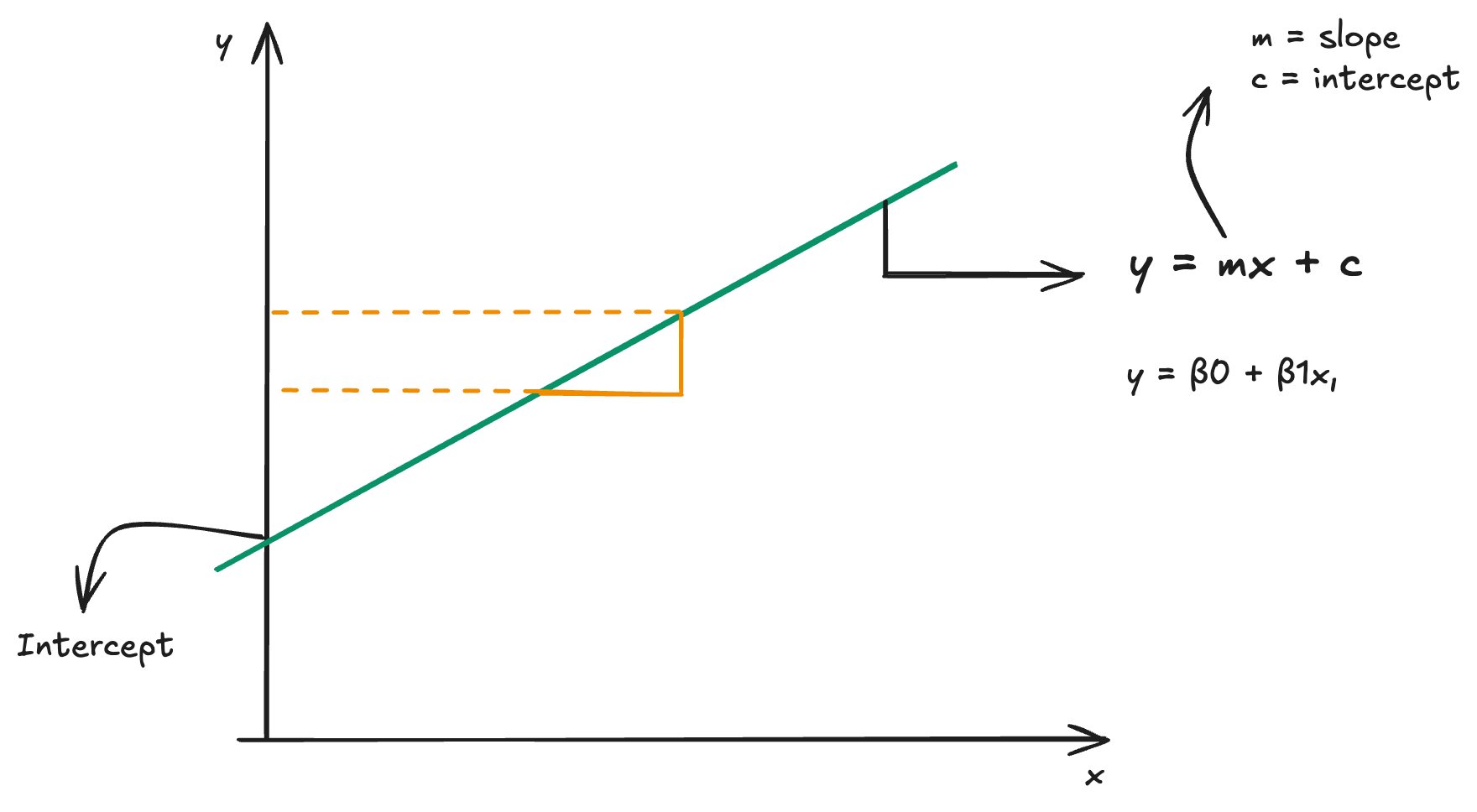
Let’s start where you already are: two axes, and . If you draw a straight line on this plane, you can describe it with the equation you learned in school:
- is the slope — it tells you how much moves for every one unit that moves. A big slope means a steep line; a slope of 0 means a flat line.
- is the intercept — it tells you where the line crosses the y-axis (i.e., the value of when ).
You may also see the exact same line written in other notations, such as:
These aren’t different lines — they’re just different ways of writing the same relationship. In fact, you can algebraically rearrange back into the familiar form (just solve for ), and you’ll find and the intercept term matches up too.
3.2 Moving Toward a Machine-Learning-Friendly Notation
In ML, we rarely use and as variable names once we have many features (a feature might be “age,” another might be “income,” another “height,” and so on). Instead of and , we relabel our axes as and — because this naming scheme easily extends to when we have more dimensions. Using this relabeling, our line becomes:
Notice this matches exactly — we’ve just renamed , (the coefficients, now called weights), , and (now called the bias).
Once you have more than one weight and more than one feature, it’s cleaner to write this using vectors instead of listing every term. We stack the weights into a vector and the features into a vector , and write:
This is the notation you will see everywhere in ML — logistic regression, SVMs, and even the single artificial neuron (the perceptron) all use this exact expression as their foundation. If you’ve come across the perceptron model, this should look familiar: a perceptron computes exactly , then passes it through an activation function. The “line” you’re learning here is the decision boundary a single artificial neuron draws.
3.3 Extending to a 3D Plane
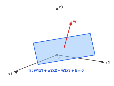
What happens when we have three axes instead of two — , , and ? We can no longer draw a straight line to split the space; instead, we need a flat sheet — a plane — cutting through 3D space. The equation naturally extends by simply adding one more term:
In vector form, this is still exactly:
— it’s just that now and each have three components instead of two. This is a great illustration of why vector notation is so powerful: the formula itself never changes as dimensions grow — only the size of the vectors inside it does.
3.4 Generalizing to N Dimensions: The Hyperplane
Now for the big generalization. What if you have features instead of just 2 or 3 (very common in real datasets — think of a dataset with 50 columns)? You simply keep extending the pattern:
which, again, compresses neatly into:
A flat “boundary” in a space with more than 3 dimensions can’t be visualized directly (our brains can’t picture 10D space), but mathematically it behaves exactly like the 2D line and 3D plane you already understand. This general object is called a hyperplane, and it is conventionally denoted using the Greek letter (pi — not the 3.14159 one!).
4. Math Section: Building the Formula Step by Step
4.1 Starting Simple: Passing Through the Origin
Let’s ask: what does it mean if our line/plane passes exactly through the origin — the point where every coordinate is 0?
If and satisfy the equation , then plugging in zeros gives:
So if a line/plane/hyperplane passes through the origin, the bias term must be exactly 0. In that special case, our general equation simplifies to:
This clean, bias-free equation is the one you’ll most often see written for hyperplanes: .
4.2 Why the Weight Vector is Perpendicular to the Plane
This is the single most important geometric insight in this whole topic, so let’s build it up carefully.
Step 1 — Recall the dot product formula from linear algebra. For any two vectors and , their dot product can be written as:
where and are the magnitudes (lengths) of the vectors, and is the angle between them.
Step 2 — Apply our plane equation. We already established that for any point lying on the plane, . Substituting this into the formula above:
Step 3 — Reason about when this can be true. Since and are (non-zero) vectors, their magnitudes and aren’t zero. The only way the whole product can equal zero is if .
Step 4 — Solve for the angle. exactly when .
Conclusion: The angle between and every single point vector that lies on the plane is exactly 90°. In plain words: the weight vector is always perpendicular (normal) to the plane it defines — no matter which point on the plane you pick.
4.3 The Geometric Picture
Think of the plane as a flat tabletop and as a rod sticking straight up out of it, like a flagpole planted perfectly upright — that “perpendicular flagpole” relationship never changes, no matter where on the table you plant it. This is why, when you see a diagram of a hyperplane in an ML textbook, the weight vector is almost always drawn as a short arrow sticking straight out of the boundary line: it’s showing you the direction the model considers “positive,” and the hyperplane is the flat surface sitting exactly perpendicular to it.
This intuition becomes critical later when studying SVMs, where the distance from a data point to the hyperplane is calculated precisely by projecting the point onto this perpendicular direction .
5. Types / Variants
Even though every case below uses the same underlying formula , the object it describes changes shape depending on how many dimensions you’re working in — much like how the same recipe produces a cookie, a cake, or a giant sheet cake depending on the pan size you use.
| Type | Dimensions of Space | Analogy | Equation |
|---|---|---|---|
| Line | 2D () | A tightrope stretched across a room | |
| Plane | 3D () | A flat sheet of glass slicing through a room | |
| Hyperplane | -D (), | An “invisible” flat boundary you can’t picture, but which behaves exactly like the line/plane above | |
| Through-origin variant | Any dimension | A boundary that’s been “recentered” so it passes exactly through the zero point | (i.e., ) |
6. Limitations and Trade-offs
Limitation: A single line/plane/hyperplane can only draw a straight, flat boundary.
Concrete example: imagine a dataset where you’re trying to separate “apples” from “oranges” based on two features (sweetness and size), but the apples happen to form a ring around a central cluster of oranges (a bullseye pattern). No matter how you rotate or shift a straight line, you cannot separate a ring shape from what’s inside it — a straight line always divides the plane into exactly two flat half-spaces, and a circular boundary simply isn’t flat.
This is a genuine limitation of relying purely on . It’s exactly the kind of problem that a plain perceptron (which can only learn straight-line/hyperplane boundaries) fails at — famously, a single perceptron cannot even learn the XOR logic gate, because XOR isn’t linearly separable.
How this was later addressed: Two major fixes emerged:
- Kernel methods (used in SVMs) mathematically project the data into a higher-dimensional space where a straight hyperplane can separate what was a curved boundary in the original space — the ring-shaped apple/orange example becomes linearly separable once lifted into 3D.
- Deep learning / multi-layer neural networks stack many perceptron-like units (each drawing its own simple hyperplane) together with non-linear activation functions, letting the network combine many straight boundaries into complex, curved decision regions.
So while the equation you learned here is “just” a straight line/plane/hyperplane, it becomes the fundamental repeated building block that more powerful models use over and over to approximate far more complex shapes.
7. Connecting the Dots (Correlating with What You Already Know)
- Perceptron / Artificial Neuron: A perceptron literally computes as its very first step (before applying an activation function). Everything you just learned about lines and hyperplanes is the perceptron’s decision boundary.
- Deep Learning: Every neuron in every layer of a deep network is computing its own little hyperplane equation on its inputs. A deep network is, geometrically, thousands of hyperplanes being combined and bent (via activation functions) to carve out very complex regions of space.
- Machine Learning Types: This topic underlies supervised learning classification tasks specifically — logistic regression and SVM both work by trying to find the best-fitting and that separate classes of labeled data using exactly this equation.
- Vectors and Dot Products (Linear Algebra): The perpendicularity result in Section 4.2 is a direct, practical payoff of the abstract dot-product formula — a nice bridge between “pure math” linear algebra and applied ML geometry.
8. Quick Recap Table
| Concept | Meaning |
|---|---|
| Slope () | How much changes per unit change in |
| Intercept ( / ) | The value of (or the offset) when all inputs are 0 |
| Weights () | The coefficients of each feature; generalized version of slope |
| Bias () | Generalized version of the intercept; shifts the boundary away from the origin |
| The general equation of a line (2D), plane (3D), or hyperplane (-D) | |
| Special case where the boundary passes through the origin () | |
| Hyperplane | The general term for a “flat” boundary in a space of any number of dimensions |
| is perpendicular to the plane | The weight vector always points in the direction normal (90°) to the boundary it defines |
| Linear separability | Whether two classes of data can be split by a straight line/plane/hyperplane |
9. Key Takeaway
The equation of a line, , is not just a 10th-grade formula — it’s the seed of one of the most powerful ideas in machine learning. By relabeling axes as and coefficients as weights , the exact same equation extends seamlessly from a 2D line, to a 3D plane, to an -dimensional hyperplane: . Geometrically, the weight vector always stands perpendicular to this boundary, pointing in the direction the model treats as “positive” — and this single equation is the literal foundation on which perceptrons, logistic regression, SVMs, and every neuron in a deep network are built.
Additional Notes
- On notation: you may encounter the same line written as , , or — these are all algebraically interchangeable, just different conventions used in different textbooks/fields (statistics often prefers the notation; ML often prefers and ).
- Matrix multiplication reminder: when computing , the transpose is necessary because both and are typically stored as column vectors — you need one of them “lying on its side” (a row vector) to perform valid matrix multiplication and get a single scalar (number) as the result, rather than a matrix.
- This topic is explicitly called out as foundational groundwork before studying logistic regression and support vector machines (SVM) — both algorithms spend their “training” process searching for the best possible and for this exact equation.