Cost Function
1. Introduction
Imagine you’re playing a game of “hot and cold” — a friend hides an object somewhere in a room, and every time you move, they tell you either “warmer” or “colder” based on how close you’re getting. You don’t get to see the object directly, but that single word — warmer or colder — is enough information to eventually walk right up to it.
Training a machine learning model works in a strikingly similar way. The model starts with a random guess for its parameters (like the slope and intercept in your Simple Linear Regression notes), and it needs some kind of “warmer/colder” signal to know whether its current guess is good or bad, and by how much. That signal is the cost function.
Formally: A cost function is a mathematical function that measures how wrong a model’s predictions are compared to the actual true values, producing a single number — the lower that number, the better the model is performing.
Without a cost function, a model has no way of knowing whether its predictions are improving or getting worse as it adjusts its parameters. It’s the compass that gradient descent (and basically every learning algorithm) uses to know which direction is “better.”
2. History
The idea of measuring “how wrong” a prediction is didn’t originate in computer science at all — it traces back, once again, to the same astronomers and mathematicians of the late 1700s and early 1800s you met in the Simple Linear Regression notes: Legendre and Gauss, trying to fit the best possible curve through noisy telescope measurements.
Their least squares method was, in essence, the very first cost function ever formalized — a way to numerically score how far a proposed line was from the real data, by summing up squared errors. For over a century, this remained mostly a statistics tool used by astronomers, economists, and scientists fitting lines and curves to physical measurements by hand.
The real shift happened in the mid-20th century, as computing machines became powerful enough to do repeated calculations automatically. In 1847, a French mathematician named Augustin-Louis Cauchy had already described a method called gradient descent — an iterative way to find the minimum of a function by repeatedly stepping in the direction of steepest decrease. But this idea sat relatively dormant for over a hundred years, because doing it by hand for anything complex was impractical.
Once computers arrived, this changed everything. In the 1950s and 60s, as early neural network research (like Frank Rosenblatt’s perceptron, which you’ve already learned about) began, researchers needed a way to automatically adjust weights based on how wrong the network’s output was. The cost function became the missing bridge: a single number a computer could calculate quickly and repeatedly, paired with gradient descent, to let a machine “learn” without a human manually tuning parameters.
From the 1980s onward, as backpropagation made it possible to compute how cost changes with respect to every weight in a deep, multi-layer network (not just a single perceptron), the cost function became the central object around which almost all of modern machine learning and deep learning revolves — every model, from simple regression to today’s largest neural networks, is fundamentally just “define a cost function, then find the parameters that minimize it.”
3. Core Concepts
3.1 The Building Blocks
| Term | Meaning |
|---|---|
| Prediction | The model’s output for a given input, based on its current parameters |
| Actual/True value | The real, observed value we’re comparing the prediction against |
| Error / Residual | The gap between prediction and actual value for one data point |
| Cost function J(θ) | A single number summarizing the total error across all data points, as a function of the model’s parameters θ |
| Parameters (θ) | The values the model is allowed to adjust — e.g., slope and intercept |
| Global minimum | The specific parameter values where the cost function is as low as it can possibly be |
3.2 Why “a Single Number” Matters
A model might have thousands, even millions, of parameters (weights and biases) in a deep network. You can’t look at all of them individually and judge “is this good?” The cost function’s entire purpose is to collapse the performance of the whole model, across every data point, into one single number — so that “better” and “worse” become simple to compare, and so that calculus (specifically, derivatives) can be used to figure out which direction to adjust each parameter in.
3.3 From Individual Error to Total Cost
This builds in three layers, each one wrapping around the previous:
- Per-point error: How wrong is the model for one specific example? (e.g., )
- Aggregation: Combine the errors across all data points into one number (usually by summing squared errors).
- Normalization: Scale that number sensibly (e.g., divide by the number of data points) so it’s comparable across different dataset sizes.
This is exactly the structure of from the previous discussion — and it’s a pattern that repeats in every cost function you’ll ever encounter, no matter how complex the model gets.
3.4 Two Notations, One Idea: θ vs. β
Right about now you might be wondering: “Wait, in the SLR notes we used , but here everyone writes — are these different things?”
They’re not. They’re the exact same slope and intercept, just written in two different notational “dialects” that come from two different traditions:
- (beta notation) comes from classical statistics — the world of Legendre, Gauss, and Galton from the History section, where regression was solved directly with a closed-form formula.
- (theta notation) comes from machine learning — the world of gradient descent, perceptrons, and neural networks, where parameters are learned iteratively rather than solved in one shot.
Since Simple Linear Regression sits at the exact crossroads of both traditions, you’ll see it written both ways depending on which textbook or course you’re reading.
| Statistics notation (SLR notes) | ML notation (this section) | Meaning |
|---|---|---|
| The intercept — predicted output when input is 0 | ||
| The slope — how much output changes per unit of input | ||
| The model’s prediction (the “hypothesis” function, in ML terms) | ||
| The -th input value | ||
| The -th actual/true output value | ||
| Total number of data points | ||
| Total error, aggregated and (in ML’s case) normalized |
Why the difference matters beyond just symbols: it’s not just relabeling — it reflects how each field expects you to find the best / values.
- In the world, since SLR’s cost surface is a simple smooth bowl with only 2 parameters, you can take derivatives, set them to zero, and solve directly — giving you the exact closed-form formulas from the SLR notes:
- In the world, the same underlying math is framed so it generalizes — the update rule works whether you have 2 parameters (like SLR) or 2 million parameters (like a deep network), because you’re not solving directly — you’re stepping downhill on the cost surface, bit by bit, using gradient descent.
The key insight: for Simple Linear Regression specifically, both roads lead to the same destination — the same best-fit line. Solving the formulas directly and running gradient descent on until it converges will give you (essentially) identical values. SLR is small and simple enough that you don’t even need gradient descent — but learning it here matters because gradient descent is the only option once your model grows into a perceptron or a deep network, where no closed-form formula exists anymore.
3.5 The Cost Surface — Visualizing “Wrongness”
If a model has just two parameters (like and in SLR), you can actually plot the cost function as a 3D surface — a bowl-shaped landscape where the height at any point tells you how bad that particular combination of parameters is. Training a model becomes the process of walking downhill on this surface until you reach the lowest point — the bottom of the bowl. This is the intuition gradient descent is built on.
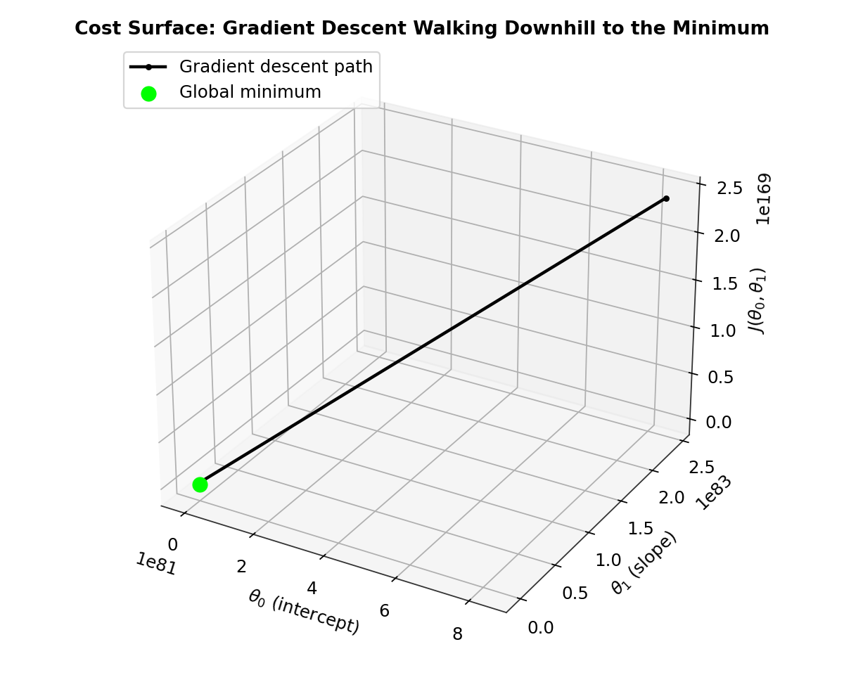
Every point on this bowl-shaped surface represents one possible combination of , and its height is the cost for that combination. The black trail is gradient descent taking repeated downhill steps, starting from a random point high on the bowl’s wall and converging toward the green dot — the global minimum, which is exactly the pair the closed-form formula would have given you directly.
4. The Math — Building It Step by Step
4.1 Step 1: Start with a Single Prediction Error
For one data point , the model predicts . The raw error is:
This can be positive (model overshot) or negative (model undershot).
4.2 Step 2: Why Squaring Is the Standard Choice
Just like in the SLR notes, if you summed raw errors directly, positive and negative errors would cancel out and hide the model’s true performance. Squaring fixes this:
Bonus reason this matters for learning specifically: squaring makes the cost function smooth and differentiable everywhere — meaning it has no sharp corners or breaks. This is essential because gradient descent relies on calculating a derivative (slope) of the cost function at every step; a jagged function would make that unreliable.
4.3 Step 3: Aggregate Across All Data Points
Sum the squared errors across every one of the training examples:
4.4 Step 4: Normalize
Divide by — by to average the error per example (so cost doesn’t blow up just because you have more data), and by an extra 2 purely to make the derivative clean later on:
This is called the Mean Squared Error (MSE) cost function (technically “half-MSE,” because of that extra ).
4.5 Step 5: How the Cost Function Actually Gets Minimized
Once is defined, the learning process (gradient descent) repeatedly updates each parameter in the direction that decreases cost the fastest:
Why this makes sense in plain words:
- is the slope of the cost surface at the current parameter values — it tells you which direction is “uphill.”
- Since you want to go downhill (toward lower cost), you subtract that slope rather than add it.
- (the learning rate) controls how big a step you take each time — too large and you might overshoot the minimum; too small and learning takes forever.
This update rule is repeated over and over — each repetition nudges and a little closer to the values that minimize .
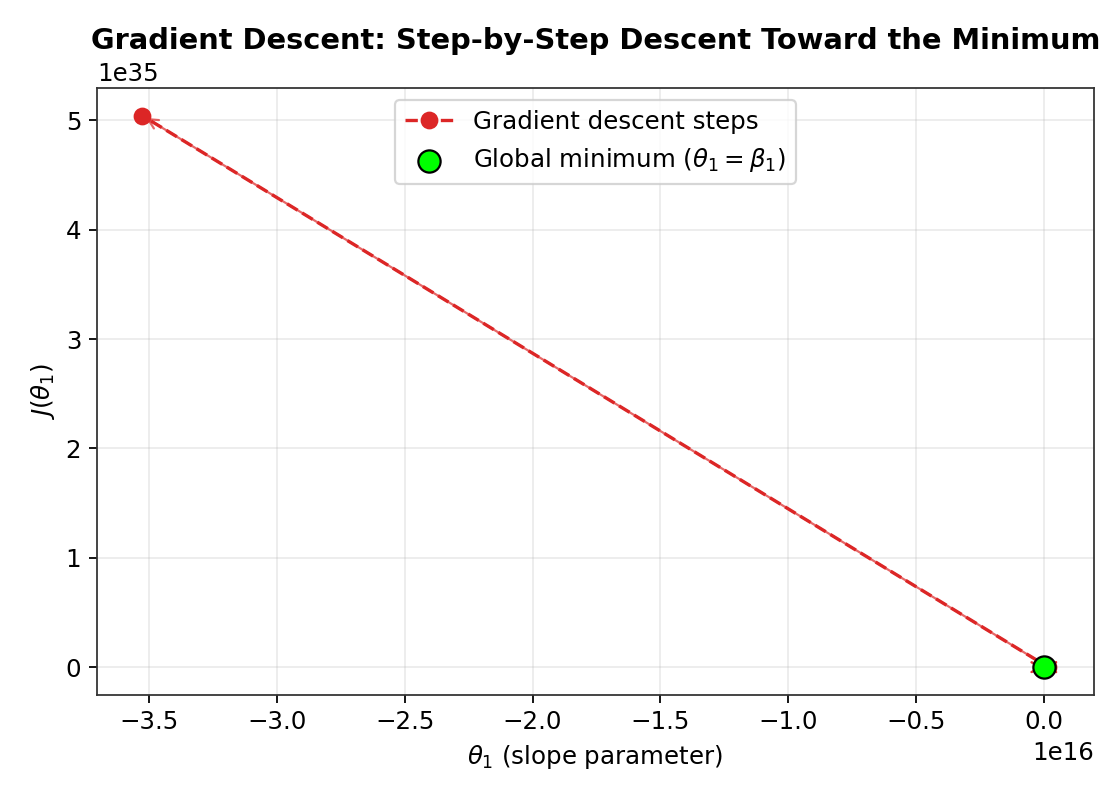 Simplifying to just one parameter () so it fits on a 2D graph: each red arrow is one gradient descent update. Notice the steps get smaller as the curve flattens near the bottom — that’s because the slope (gradient) itself gets smaller closer to the minimum, so each update naturally shrinks even though stays fixed.
4.6 Geometric Interpretation
Picture the bowl-shaped 3D surface from section 3.4 again. The gradient (the partial derivative) at any point tells you the direction of steepest ascent on that surface. Gradient descent simply walks in the opposite direction, step by step, learning-rate-sized stride by stride, spiraling down toward the bottom of the bowl — the point where is smallest, which corresponds to the best-fitting parameters.
5. Types / Variants of Cost Functions
Different problems need different ways of measuring “wrongness,” because not every kind of error should be penalized the same way.
- Mean Squared Error (MSE) is like a strict teacher who deducts exponentially more marks the further off your answer is — being slightly wrong costs a little, being very wrong costs a lot.
- Mean Absolute Error (MAE) is like a fairer teacher who deducts marks proportionally to how wrong you are, without extra punishment for being very wrong — treating a huge miss and several small misses as comparable if their total distance is the same.
- Cross-Entropy / Log Loss is like a teacher grading a yes/no quiz, who penalizes you severely for being confidently wrong (saying “definitely yes” when the answer was no) but barely penalizes you for being unsure.
- Huber Loss is like a teacher who’s fair (like MAE) for big mistakes but strict (like MSE) for small ones — a deliberate hybrid to get the best of both.
| Cost Function | Used For | Sensitivity to Outliers | Analogy |
|---|---|---|---|
| Mean Squared Error (MSE) | Regression (predicting numbers) | High — large errors punished heavily | Strict teacher, penalty grows with the square of the mistake |
| Mean Absolute Error (MAE) | Regression | Low — errors punished proportionally | Fair teacher, penalty grows linearly |
| Cross-Entropy / Log Loss | Classification (predicting categories) | Punishes confident wrong answers heavily | Quiz grader who hates confident incorrect guesses |
| Huber Loss | Regression, especially with some outliers | Medium — behaves like MAE far away, MSE close up | A hybrid teacher — fair on big misses, strict on small ones |
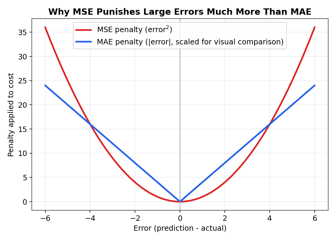
Notice the shapes: MSE’s penalty (red) curves upward — doubling the error more than doubles the penalty. MAE’s penalty (blue) grows in a straight line — doubling the error exactly doubles the penalty. This is precisely why MSE is far more sensitive to outliers than MAE, as explained in the next section.
6. Limitations and Trade-offs
6.1 MSE’s Sensitivity to Outliers
Worked example: Suppose you’re predicting house prices and your model is off by ₹1 lakh on nine houses, but off by ₹50 lakh on one unusual mansion (bad data or a genuine anomaly). Because MSE squares errors, that one ₹50 lakh error contributes (in squared units) to the cost, while each ₹1 lakh error only contributes . That single outlier can dominate the entire cost function, pulling the model’s parameters toward accommodating the mansion at the expense of accuracy on the other nine houses — the exact same outlier problem you saw with SSE in the SLR notes, because MSE and SSE are built from the same squared-error idea.
Fix that came later: This is exactly why MAE and Huber Loss were developed — to reduce the outsized influence of extreme outliers.
6.2 Choosing the Wrong Cost Function for the Task
Worked example: Imagine using MSE for a spam-detection model (a classification task: spam or not spam) instead of cross-entropy. MSE treats a prediction of “70% confident it’s spam” as only mildly different from “51% confident” — it doesn’t strongly discourage the model from sitting on the fence. Cross-entropy, by contrast, sharply penalizes confidently wrong predictions, which is far more useful for pushing a classifier to make decisive, well-calibrated decisions. Using the wrong cost function doesn’t just slow learning down — it can make the model converge to genuinely worse parameters for the task at hand.
6.3 Non-Convex Cost Surfaces (Getting Stuck)
For simple models like SLR, the cost surface is a smooth, single bowl (convex), so gradient descent is guaranteed to find the true lowest point. But for deep neural networks with many layers, the cost surface can have multiple dips and valleys (non-convex), meaning gradient descent can get stuck in a “local minimum” — a point that looks like the bottom locally, but isn’t the true lowest point overall.
Fix that came later: Techniques like momentum, adaptive learning rates (Adam optimizer), and random restarts were developed to help gradient descent escape shallow local minima and find better solutions in these more complex, non-convex landscapes.
7. Connecting to What You Already Know
The Simple Linear Regression connection: The cost function you just learned, , is the exact same object as the SSE formula from your SLR notes — just averaged (divided by ) and rescaled (divided by 2) to make gradient descent’s calculus cleaner. SLR can be solved with a closed-form formula precisely because its cost function is simple enough to solve directly; more complex models can’t do that and must rely on iteratively minimizing the cost function instead.
The perceptron connection: A perceptron adjusts its weights based on how wrong its output was for each example — this “how wrong” measurement is a cost function. Early perceptron learning rules were, in effect, primitive cost-minimization procedures, refined later into the more general gradient descent framework used today.
The biological neuron connection: Just as your earlier notes compared a perceptron’s weighted sum to a neuron combining signals, you can think of the cost function as biology’s version of a “pain/pleasure” or feedback signal — a single measurable quantity that tells a learning system whether its recent behavior should be reinforced or corrected, guiding future adjustments.
The deep learning connection: In deep neural networks, the same core idea — define a cost function, then minimize it — still applies, just scaled up massively. Instead of adjusting 2 parameters () like in SLR, deep learning models adjust millions or billions of weights simultaneously, using backpropagation to efficiently compute the gradient of the cost function with respect to every single one of those weights, layer by layer.
The machine learning types connection: The choice of cost function is directly tied to the type of supervised learning problem: regression problems (predicting numbers, like SLR) typically use MSE or MAE, while classification problems (predicting categories, like logistic regression) typically use cross-entropy — reinforcing that the cost function isn’t one-size-fits-all, but chosen based on what kind of output the model produces.
8. Quick Recap Table
| Concept | Meaning |
|---|---|
| Cost function J(θ) | A single number measuring how wrong a model’s predictions are, as a function of its parameters |
| Hypothesis h_θ(x) | The model’s prediction function |
| Error/Residual | Difference between prediction and actual value for one example |
| Mean Squared Error (MSE) | Average of squared errors — the most common regression cost function |
| Learning rate (α) | Controls the step size when updating parameters during gradient descent |
| Gradient descent | Iterative algorithm that adjusts parameters to minimize the cost function, step by step |
| Cost surface | The 3D “landscape” formed by plotting cost against parameter values |
| Global minimum | The lowest possible point on the cost surface — the ideal parameter values |
| Local minimum | A point that looks lowest nearby but isn’t the true lowest point overall (a risk in non-convex surfaces) |
| Cross-entropy/Log loss | Cost function used for classification, punishing confident wrong predictions heavily |
| Convex vs. non-convex | Whether the cost surface is a single smooth bowl (convex, easy to minimize) or has multiple dips (non-convex, harder) |
9. Key Takeaway
A cost function is the single number that tells a learning algorithm whether it’s getting better or worse — it’s the “warmer/colder” signal that turns blind parameter-guessing into directed learning. Every model you’ll encounter, from Simple Linear Regression’s closed-form least squares solution to a perceptron’s weight updates to a massive deep neural network trained with backpropagation, is ultimately doing the same fundamental thing: defining some measure of “wrongness” as a cost function, then using calculus (via gradient descent) to walk downhill on that cost surface until the parameters that minimize error are found.