MSE, MAE and RMSE
1. Introduction
Imagine you’ve just built a Simple Linear Regression model predicting salary from years of experience. You plot your data points — years of experience on the X-axis, salary on the Y-axis — and draw your best-fit line through them. For every person in your dataset, the line gives a predicted salary (), while their actual salary is the truth value (). Naturally, some predictions are spot-on, some are a little off, and some might be quite far off.
Now here’s the real question: how do you put a single number on “how good is this line, overall”? You already know from your earlier notes that and Adjusted answer a version of this question — but those give you a broad performance score. If you want to focus specifically on the error at each individual data point and combine it meaningfully, you need a different toolkit: MSE (Mean Squared Error), MAE (Mean Absolute Error), and RMSE (Root Mean Squared Error).
Formally: MSE, MAE, and RMSE are all “error metrics” — ways of aggregating the gap between predicted and actual values across an entire dataset into one number that tells you how wrong your model typically is. They’re not three unrelated ideas; they’re three different ways of answering the exact same question, each with its own trade-offs — which is exactly what this note will unpack.
2. History
These three metrics all trace back to the same root you’ve already met in your Simple Linear Regression notes: Legendre and Gauss’s least squares method from the early 1800s. Squaring the error to get rid of cancelling positive/negative signs — the same trick from your SLR notes — is precisely what MSE is built on, so in a real sense, MSE isn’t a separate invention; it’s simply the “least squares” idea repackaged as an average rather than a raw sum, so it can be compared fairly across datasets of different sizes.
Mean Absolute Error grew out of a long-running tension in statistics: least squares (squared error) is mathematically convenient, but statisticians noticed early on that it reacts very badly to extreme, unusual observations. Alternatives based on absolute differences — rather than squared ones — had actually been explored even before Legendre’s 1805 publication, by figures like Roger Boscovich in the 1760s, precisely because absolute error is naturally more resistant to being thrown off by a handful of extreme points. For a long time, though, squared-error approaches dominated practice simply because they were easier to solve by hand with calculus — you’ll see exactly why in the math section below.
Root Mean Squared Error emerged as a practical patch on MSE’s biggest annoyance: units. As computing and statistics matured through the 20th century and these metrics moved from academic papers into everyday engineering and business use, practitioners needed error numbers that were directly interpretable in the same units as the original data (like “lakhs of salary,” not “lakhs-squared”). Taking the square root of MSE was the natural fix — mathematically trivial, but practically important, and RMSE became the standard “headline” error metric reported for regression models across many fields, from weather forecasting to finance.
3. Core Concepts
3.1 The Building Blocks
Picture the salary-vs-experience example from the Introduction as your reference throughout these notes.
| Term | Meaning |
|---|---|
| Truth value (y) | The actual, observed value — e.g., a person’s real salary |
| Predicted value (ŷ) | The value your model’s best-fit line predicts for that same input |
| Error / Residual | The gap between truth and prediction: |
| n | The total number of data points in your dataset |
| Cost function / Loss function | A formula that aggregates all the individual errors into one overall score |
3.2 Recap: Where This Connects to Gradient Descent
You’ve already seen in your Cost Function notes that training a linear regression model means minimizing a cost function using gradient descent, walking step by step toward the global minima — the point where the cost is as low as possible. MSE, MAE, and RMSE are exactly the candidate cost functions you could plug into that same process. Which one you choose changes how the gradient descent journey behaves — as you’ll see clearly in the next few sections.
4. Mean Squared Error (MSE)
4.1 Building the Formula
Start with the raw error for a single data point: . Since some errors are positive (under-prediction) and some negative (over-prediction), simply adding them up lets errors cancel out, hiding the model’s true performance — the same issue you saw when deriving the least-squares formula in your SLR notes.
Fix: square each error. This makes every term positive, so nothing cancels, and (as a bonus) it punishes bigger mistakes disproportionately more than small ones.
Averaging these squared errors across all data points gives you:
This is the exact same formula as the cost function from your earlier notes (aside from the constant some versions include purely to simplify the derivative during gradient descent) — MSE is the least-squares cost function, just given its own standalone name as a performance metric.
4.2 Why MSE’s Shape Makes It So Convenient
Here’s a neat algebraic observation: , when squared, expands using the identity . This is precisely the structure of a quadratic equation — and if you plot a quadratic equation, you get a smooth, bowl-shaped (convex) curve. This bowl shape is exactly the “cost surface” you visualized in your Cost Function and Convergence notes, and it’s the reason gradient descent works so cleanly with MSE.
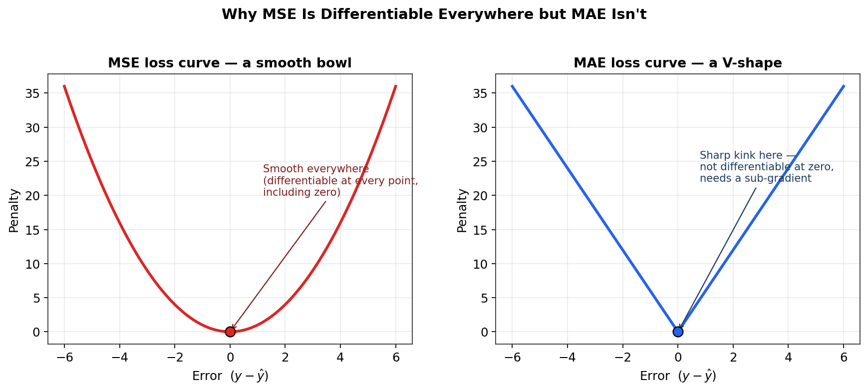
Two loss curves side by side: MSE forms a smooth bowl-shaped quadratic curve differentiable everywhere, while MAE forms a V-shape with a sharp kink at zero
The left curve (MSE) is smooth at every single point, including right at zero — there’s no sharp corner anywhere. This matters enormously for training, as the next section explains.
This gives MSE three genuine advantages:
- Differentiable everywhere. Because the curve has no sharp corners, you can calculate a derivative (a slope) at every point on it — including exactly at the minimum. This is essential for gradient descent, which relies on computing that slope at each step to know which direction to move in.
- Exactly one global minimum, no local minima. A quadratic curve like this is what’s called a convex function — it only ever has a single dip. Contrast this with a non-convex function, which can have multiple dips (local minima) alongside the true lowest point (the global minimum). If gradient descent gets stuck in a local minimum, it wrongly believes it has finished training (because the slope is zero there too), even though a better solution exists elsewhere. Because MSE’s curve is convex, this trap simply can’t happen — there’s only one minimum, and it’s always the global one.
- Faster convergence. Precisely because there’s no risk of getting trapped in a local minimum, and the curve is smooth and predictable, gradient descent tends to reach the minimum for MSE more reliably and efficiently than for less well-behaved cost functions.
4.3 MSE’s Disadvantages
Disadvantage 1 — Not robust to outliers. Because MSE squares every error, an unusually large error gets penalized disproportionately — this is called penalizing the outlier.
Worked example: Picture your salary-vs-experience data forming a tidy, roughly straight cluster, with a well-fitted best-fit line running through the middle. Now suppose a new data point comes in that’s a genuine outlier — say, someone with 9.5 years of experience but a salary far higher than the trend would predict.
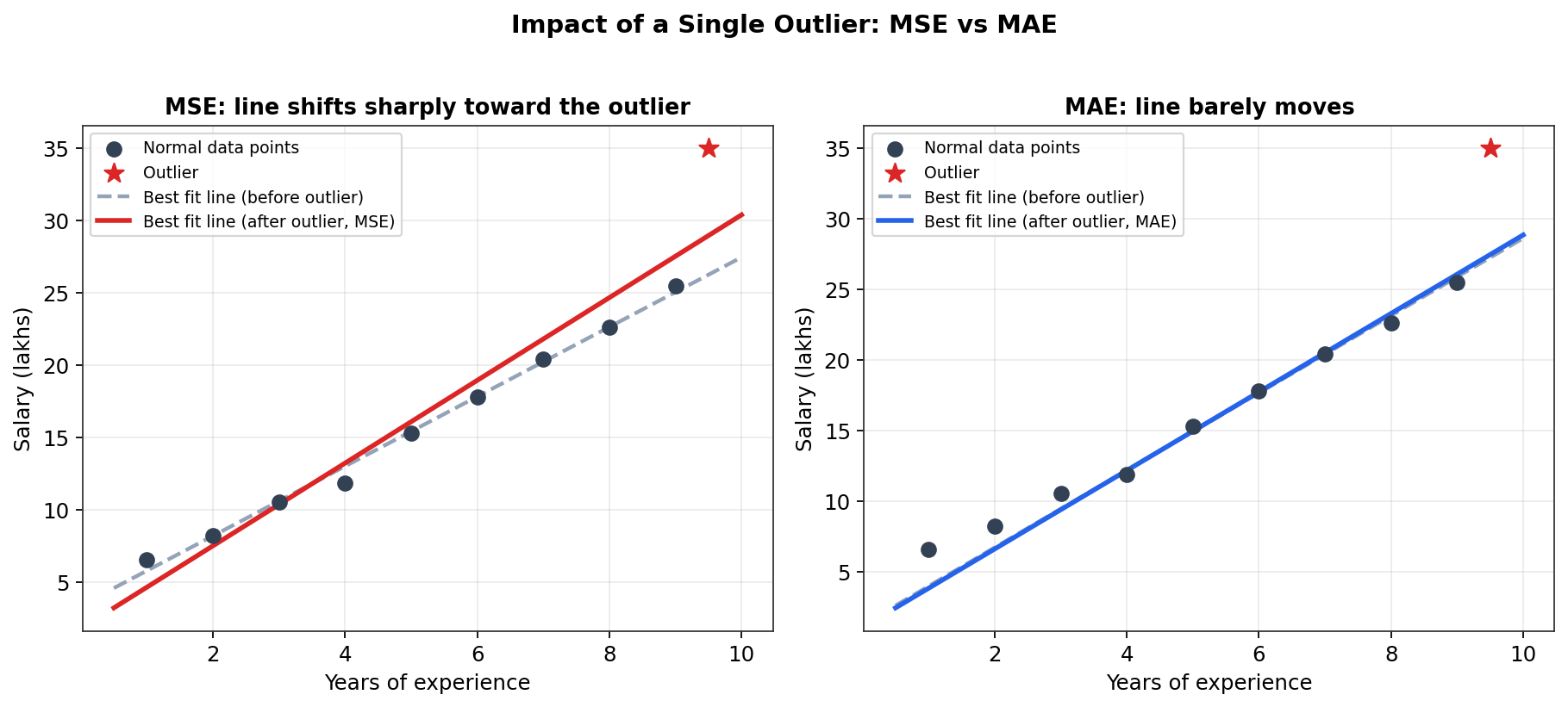
Two scatter plots comparing how a single outlier shifts the best-fit line under MSE versus MAE; the MSE line swings sharply toward the outlier while the MAE line barely moves
On the left, notice how dramatically the red MSE-fitted line tilts away from the grey “before outlier” line, chasing the outlier at the expense of accuracy on all the normal points. Because MSE squares that one large error, minimizing MSE forces the line to move substantially to reduce that squared penalty — even though doing so makes the line noticeably worse for every other point.
Disadvantage 2 — Loses the original units. Suppose salary is measured in lakhs. When you compute , you’re not just measuring an error in lakhs anymore — you’re measuring it in lakhs², or “lakhs squared.” If your MSE comes out to, say, 2.5, that’s 2.5 lakhs² — a number that’s mathematically valid but practically hard to interpret directly against the original salary values. This mismatch in units is the direct motivation for RMSE, covered next.
5. Mean Absolute Error (MAE)
5.1 Building the Formula
MAE takes a different approach to solving the “cancel-out” problem from section 4.1: instead of squaring the error, it takes the absolute value:
Every term is guaranteed non-negative (since absolute value strips the sign), so errors still can’t cancel out — but unlike squaring, absolute value doesn’t disproportionately amplify large errors. A error twice as large contributes exactly twice as much to MAE, not four times as much like it would with MSE.
5.2 MAE’s Advantages
Advantage 1 — Robust to outliers. Going back to the same salary outlier example: since MAE doesn’t square the error, one unusually large mistake increases the total error only by its own size, not by its square.
Looking back at the right-hand panel of the outlier diagram above: the blue MAE-fitted line stays much closer to the grey “before outlier” line — the shift caused by the exact same outlier is far smaller than what MSE produced. This is precisely why MAE is described as robust to outliers — a handful of extreme points simply can’t dominate the fit the way they can under MSE.
Advantage 2 — Same units as the original data. Since there’s no squaring involved, stays in the same units as itself — lakhs stay lakhs, not lakhs². This makes MAE values much more directly interpretable at a glance.
5.3 MAE’s Disadvantage
Not differentiable at zero. Plot the absolute value function, and you’ll notice it forms a clean V-shape — but right at the point where the error is zero, there’s a sharp corner (see the right-hand curve in the differentiability diagram in section 4.2). A sharp corner has no single well-defined slope — you genuinely cannot differentiate a function at a point where it has a kink.
In practice, this is worked around using sub-gradients — a mathematical patch that essentially picks a reasonable slope value from a valid range at that problematic point, rather than a single exact derivative. It works, but it introduces extra complexity into the optimization process. As a direct consequence, gradient descent using MAE as its cost function tends to converge more slowly than it does with MSE, since the smooth, predictable “always know exactly which way is downhill” behavior of MSE isn’t fully available near the minimum.
6. Root Mean Squared Error (RMSE)
6.1 Building the Formula
RMSE is built directly on top of MSE — it’s simply the square root of it:
Why this makes sense in plain words: squaring the error (to get MSE) changed its units from “lakhs” to “lakhs²,” as you saw in section 4.3. Taking the square root is the mathematically clean way to undo exactly that unit-change and bring the error metric back down to the original, interpretable scale — while still keeping all the benefits of the squaring trick (no cancellation, smooth differentiability) baked into the calculation underneath.
6.2 RMSE’s Advantages and Disadvantages
Advantage — Same units as the original data, just like MAE, but achieved differently: by unwinding the square rather than avoiding it in the first place.
Advantage — Still differentiable, since it’s built from the same smooth quadratic MSE curve underneath (with the square root applied afterward), so it retains gradient descent’s smooth, well-behaved convergence properties.
Disadvantage — Still not robust to outliers. Since RMSE is fundamentally still built on squared errors internally, it inherits MSE’s core weakness — a large outlier still gets squared and disproportionately amplified before the square root is applied at the very end, so the underlying sensitivity to extreme values doesn’t actually go away; only the final unit gets corrected.
7. R² (R-squared): Putting the Error in Context
7.1 Why You Need This on Top of MSE, MAE, and RMSE
Here’s a gap in everything covered so far: if someone tells you “my model’s MSE is 4.2,” is that good? You genuinely can’t tell — it depends entirely on the scale of your data. An MSE of 4.2 might be excellent for predicting salaries in crores, but terrible for predicting a probability between 0 and 1. MSE, MAE, and RMSE all measure how wrong your model is in absolute terms, but none of them tell you how that compares to not having a model at all.
R² (R-squared), also called the coefficient of determination, fills exactly this gap — it’s a unitless score that tells you how much better your regression line is than the simplest possible baseline: just predicting the mean of every time.
7.2 Building the Formula
Step 1 — Your model’s actual error (): this is simply before averaging — the same sum-of-squared-residuals idea from your SLR notes and from section 4.1 above:
Step 2 — The “dumb baseline” error (): how wrong you’d be if you ignored entirely and just guessed the mean every time:
Step 3 — Compare them:
Why this makes sense in plain words: is “how much error your model still has, relative to the dumb baseline’s error.” Subtracting that fraction from 1 flips it into “how much of the baseline’s error your model managed to eliminate.”
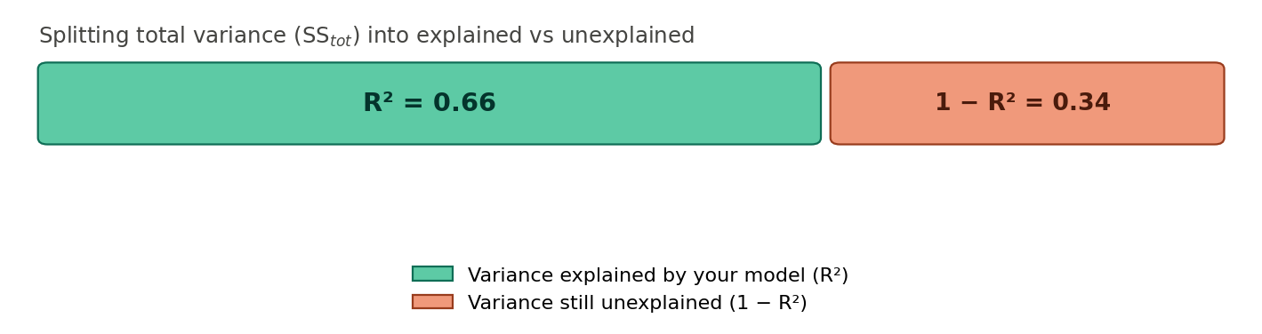
Bar split into a teal segment labeled R squared 0.66 representing variance explained by the model, and a coral segment labeled 1 minus R squared 0.34 representing variance still unexplained
Picture the total variance in your salary data as one full bar. Fitting your regression line “explains away” part of that variance (teal) — the rest (coral) is error your line still couldn’t account for. R² is simply the teal fraction.
7.3 Reading the Value
- : your line predicts perfectly — , so 100% of the variance is explained.
- : your line is no better than just guessing the mean — it isn’t picking up any real relationship between and .
- (yes, this can happen): your fitted line is somehow worse than the dumb baseline — a real possibility with a badly fit or badly chosen model.
7.5 Adjusted R²
Adjusted R² is a modified version of R² that penalizes you for adding predictors that don’t actually help the model.
The problem with plain R²
Regular R² measures how much variance in y is explained by your model:
where (residual sum of squares) and (total sum of squares).
The issue: R² never decreases when you add more features — even totally useless, random ones. Add enough junk predictors and R² will keep creeping toward 1, making your model look better than it really is. This is misleading, especially when comparing models with different numbers of features.
The fix: Adjusted R²
where:
- n = number of data points (sample size)
- k = number of predictors (independent variables), not counting the intercept
What it does differently
Adjusted R² adds a penalty term based on the number of predictors relative to the sample size. If a new feature actually improves the model meaningfully, adjusted R² increases. If you add a feature that’s essentially noise, adjusted R² decreases — even though plain R² would still go up (or stay flat).
Quick intuition
| Scenario | R² | Adjusted R² |
|---|---|---|
| Add a genuinely useful predictor | ↑ | ↑ |
| Add a useless/random predictor | ↑ (slightly) | ↓ |
| Add a predictor with zero relationship to y | stays same or ↑ tiny | ↓ |
Why it matters
- Use R² to describe how well your current model fits the data.
- Use Adjusted R² when comparing models with different numbers of features — it tells you whether adding a variable was actually worth it, or if you’re just overfitting.
It’s especially important in multiple linear regression, where it’s tempting to throw in lots of features hoping to boost R².
7.4 How R² Connects Back to MSE, MAE, and RMSE
in the R² formula is exactly — so R² is really answering “how much smaller is my MSE than the MSE I’d get from just guessing the mean?” This is why R² and the three error metrics are used together rather than as substitutes: MSE/MAE/RMSE tell you the size of your error in the original problem’s terms, while R² tells you how meaningful your model is relative to doing nothing at all. A model can have a small RMSE in absolute terms but a poor R² if the underlying data itself has very little natural variance to explain — the two numbers genuinely answer different questions.
One quick caveat worth knowing (Adjusted R²): plain R² has a quirk — it never decreases when you add more input variables to a model, even completely useless ones, which can make a model look artificially better than it is. Adjusted R² corrects for this by penalizing the score for unnecessary added variables, making it the fairer choice specifically when comparing models with different numbers of inputs — though since Simple Linear Regression only ever has one input variable, plain R² and Adjusted R² will always agree for the models discussed in these notes.
8. Comparing All Three
| Metric | Formula | Same units as data? | Robust to outliers? | Differentiable everywhere? | Convergence speed |
|---|---|---|---|---|---|
| MSE (Mean Squared Error) | No (units²) | No | Yes | Fast | |
| MAE (Mean Absolute Error) | Yes | Yes | No (kink at zero) | Slower | |
| RMSE (Root Mean Squared Error) | Yes | No | Yes | Fast |
Analogies for each:
- MSE is like a strict examiner who doesn’t just deduct marks for a wrong answer, but deducts exponentially more the further off you were — one badly wrong answer can tank your entire score.
- MAE is like a fair examiner who deducts marks proportionally to how wrong you were, with no extra penalty for being very wrong — a consistent, forgiving grading scheme.
- RMSE is like the strict examiner from MSE, except the final score gets rescaled back down to a familiar, easy-to-read grading scale — same strictness underneath, friendlier number on the surface.
9. Limitations and Trade-offs — Putting It All Together
The core trade-off across all three metrics is a genuine tug-of-war between robustness and optimization convenience:
- Squared-error approaches (MSE, RMSE) are easy and reliable to optimize (smooth, single global minimum, fast convergence) but get thrown off badly by outliers, and MSE alone loses interpretable units.
- The absolute-error approach (MAE) is naturally resistant to outliers and keeps interpretable units, but is harder and slower to optimize because of that non-differentiable kink at zero.
Worked example tying it together: using the same salary-vs-experience dataset, if your data is mostly clean but contains one obvious data-entry mistake (say, a salary typo with an extra zero), an MAE-based model will barely notice it and stay close to the “true” underlying trend — while an MSE- or RMSE-based model will visibly warp its best-fit line trying to accommodate that single bad point, exactly as shown in the outlier diagram in section 4.3.
No universal fix — just informed choice. Unlike some earlier limitations in your other notes (where a “later fix” like Adam optimizer resolved the issue), there’s no single metric that’s strictly the best. In practice, most real-world workflows compute all three (alongside and Adjusted ) and interpret them together, rather than picking just one and ignoring the others.
10. Connecting to What You Already Know
The Simple Linear Regression connection: MSE is literally the same formula as the SSE-based cost function from your SLR notes, just averaged by instead of summed outright — the “penalizing the outlier” behavior you just learned is the same squared-residual mechanic from the geometric-squares diagram in those notes, just now framed as a standalone evaluation metric rather than purely a training objective.
The Cost Function and Convergence connection: the differentiability and convexity properties discussed here are exactly why your Cost Function notes described the SLR cost surface as a clean, single bowl-shaped 3D surface — that shape is a direct consequence of choosing MSE as the cost function. Swapping in MAE instead would produce a cost surface with a sharp crease running through it, which is part of why the convergence behavior (and the choice of learning rate from your Convergence notes) can behave differently depending on which error metric is being minimized.
The perceptron and deep learning connection: deep learning models routinely choose between MSE-style and MAE-style loss functions (and hybrids like Huber Loss, mentioned in your Cost Function notes) for the exact same reasons discussed here — outlier sensitivity versus ease of optimization — just scaled up from a two-parameter SLR model to networks with millions of weights trained via backpropagation.
The machine learning types connection: MSE, MAE, and RMSE are all metrics for regression problems specifically (predicting continuous numbers) — reinforcing the same regression-vs-classification distinction from your earlier notes, where classification problems instead lean on metrics like cross-entropy/log loss.
11. Quick Recap Table
| Concept | Meaning |
|---|---|
| MSE (Mean Squared Error) | Average of squared errors — fast to optimize, not robust to outliers, loses original units |
| MAE (Mean Absolute Error) | Average of absolute errors — robust to outliers, keeps original units, slower to optimize |
| RMSE (Root Mean Squared Error) | Square root of MSE — restores original units, still not robust to outliers |
| Differentiable | A function whose slope can be calculated at every point — true for MSE and RMSE, not fully true for MAE (kink at zero) |
| Convex function | A function with exactly one dip (one global minimum, no local minima) — MSE and RMSE are convex |
| Local minima | A point that looks like the lowest point nearby, but isn’t the true overall minimum |
| Global minima | The single true lowest point of a cost function — what gradient descent aims to reach |
| Robust to outliers | A metric whose value isn’t disproportionately dominated by a small number of extreme data points — true for MAE, not for MSE/RMSE |
| Sub-gradient | A workaround used to handle non-differentiable points (like MAE’s kink at zero) during optimization |
| Penalizing the outlier | The effect of squaring an error, which makes large errors contribute disproportionately more to the total |
| R² (R-squared) | A unitless score (0 to 1, can go negative) showing how much of the data’s variance your model explains compared to just guessing the mean |
| SS_res | Sum of squared residuals — your model’s actual remaining error; equal to MSE |
| SS_tot | Sum of squared deviations from the mean — the error of the “dumb baseline” model |
| Adjusted R² | R², corrected to penalize unnecessary extra input variables — fairer when comparing models with different numbers of inputs |
12. Key Takeaway
MSE, MAE, and RMSE are three different lenses on the exact same underlying question — “how wrong is my model, on average?” — and the differences between them boil down to one core trade-off: squaring the error (MSE, and by extension RMSE) gives you a smooth, easy-to-optimize, single-global-minimum cost surface at the cost of being easily thrown off by outliers and losing interpretable units, while taking the absolute value (MAE) gives you outlier-robustness and interpretable units at the cost of a trickier, slower optimization process. R² then adds the missing piece of context — turning a raw error number into a sense of how meaningful your model actually is compared to doing nothing at all. In practice, there’s no single “best” choice — a careful model builder reports and interprets all four together, choosing which to prioritize based on whether their dataset is clean or outlier-prone, and whether training speed, robustness, or interpretability matters most for the problem at hand.