Overfitting and Underfitting
1. Introduction
Imagine a student preparing for a math exam. One student, Student A, barely studies — they skim the textbook once and walk in knowing only the vaguest idea of how to solve problems. Unsurprisingly, they do poorly, not just on the exam but even on the practice questions they’d already seen in class.
Student B takes a very different, but equally flawed, approach: they memorize the exact practice questions and their exact answers, word for word, number for number — without understanding the underlying method. On the practice set, they score perfectly. But the moment the real exam has even slightly different numbers or phrasing, they’re lost — because they never learned the actual technique, just the specific answers.
Student C does it right — they understand the underlying method well enough to solve the practice questions and handle new, unseen questions on the real exam.
This is precisely the problem overfitting and underfitting describe in machine learning. Student A represents underfitting — a model too simple to even learn the pattern in the data it’s trained on. Student B represents overfitting — a model so obsessed with matching its training data exactly that it fails to generalize to new, unseen data. Student C represents the goal: a model that learns the actual underlying pattern well enough to generalize.
Formally: Underfitting occurs when a model is too simple to capture the real pattern in the data, performing poorly even on the data it was trained on. Overfitting occurs when a model is too complex, effectively memorizing the training data — including its noise and quirks — so it performs great on training data but poorly on new, unseen data.
2. History
The tension between underfitting and overfitting isn’t a modern machine learning invention — it’s really a specific case of a much older idea in statistics and philosophy: the bias-variance tradeoff, and even older than that, a principle called Occam’s Razor, dating back to the 14th-century philosopher William of Ockham, who argued that among competing explanations, the simplest one that fits the facts should usually be preferred.
As regression techniques (like the least-squares method from Legendre and Gauss you’ve already met in your SLR notes) became widely used through the 1800s and 1900s, statisticians began noticing an odd pattern: a curve that fit historical data perfectly sometimes made worse predictions on new data than a simpler curve that fit the historical data only loosely. This puzzled early statisticians, because intuitively, a “better fit” to known data feels like it should always mean a “better model.” The resolution came gradually through the 20th century, as statisticians formalized the idea that a model isn’t just approximating the data you have — it’s implicitly approximating a broader, unseen pattern, and matching your specific sample too exactly can actually work against that broader goal.
The term overfitting itself became common vocabulary specifically as computers made it easy to fit increasingly flexible, high-degree curves and later neural networks to data — the mathematical capability to fit any dataset (even one that’s mostly noise) arrived long before the discipline to know when to stop taking advantage of it. This became especially pressing in the 1980s and 90s, as neural networks (built from stacks of perceptron-like units, as covered in your Cost Function notes) grew large enough to have millions of adjustable parameters — far more parameters than there were training examples in many real datasets. Researchers found that unless deliberately restrained, these networks would essentially memorize their training data, hitting near-zero training error while performing terribly on new inputs.
This drove the development of a whole toolbox of countermeasures — including regularization techniques in the 1970s–90s (which penalize overly complex models mathematically), cross-validation (systematically testing on held-out data), and later dropout (introduced in 2014, specifically for neural networks, randomly “turning off” neurons during training to prevent them from over-relying on any single memorized pattern). Together, these turned overfitting from an unavoidable hazard of powerful models into a manageable, well-understood trade-off that’s now a standard part of training any machine learning model.
3. Core Concepts
3.1 The Building Blocks
| Term | Meaning |
|---|---|
| Training data | The data a model learns from directly |
| Test data / Validation data | New, unseen data used to check if the model actually generalizes |
| Generalization | A model’s ability to perform well on new data it wasn’t trained on |
| Model complexity | Roughly, how flexible or expressive a model is — how many parameters it has, or how curvy a shape it can fit |
| Underfitting | Model too simple; poor performance on both training and test data |
| Overfitting | Model too complex; great performance on training data, poor performance on test data |
| Noise | Random, meaningless fluctuation in data that isn’t part of the true underlying pattern |
3.2 Seeing It Visually
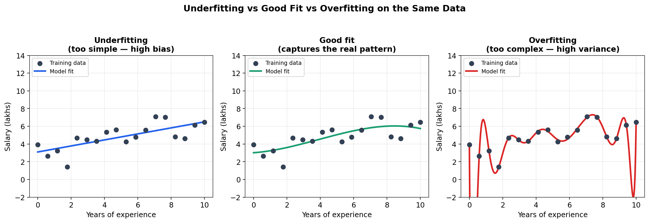
Let’s return to your salary-vs-experience example from the MSE/MAE/RMSE notes. Suppose the true underlying relationship between experience and salary isn’t perfectly linear — maybe salary growth slightly tapers off at higher experience levels, plus there’s some natural randomness (noise) in any real salary dataset.
Three side-by-side scatter plots comparing underfitting with a straight line that misses the curve, a good fit with a moderate curve matching the pattern, and overfitting with a wildly wiggly curve passing through nearly every point
Left: a straight line (like Simple Linear Regression) is too rigid to capture the slight curve in the true pattern — this is underfitting. Middle: a moderately flexible curve captures the real shape of the relationship without chasing every bit of noise — this is a good fit. Right: an extremely flexible curve contorts itself to pass through nearly every single training point, including the random noise — this is overfitting. Notice it looks “best” on the training points, but that wild wiggling would make terrible predictions for any new data point.
3.3 Training Error vs. Test Error — The Real Diagnostic
You can’t always tell overfitting from underfitting just by looking at a curve — with high-dimensional data (many input variables), there’s no simple 2D plot to eyeball. Instead, the standard diagnostic is comparing performance (using metrics like MSE, MAE, or RMSE from your earlier notes) on training data versus performance on held-out test/validation data:
| Situation | Training error | Test error |
|---|---|---|
| Underfitting | High | High (roughly similar to training error) |
| Good fit | Low | Low (close to training error) |
| Overfitting | Very low | High (much worse than training error) |
The telltale sign of overfitting specifically is a large gap between training error and test error — the model looks fantastic on data it has already seen, but that success doesn’t carry over.
4. The Math — Building the Bias-Variance Decomposition
4.1 Step 1: What Is “Error,” Really?
For any model’s prediction at some new input, statisticians decompose the expected squared prediction error (using the same squared-error idea from your MSE notes) into three distinct sources:
4.2 The Simplest Way to Picture It: Darts on a Dartboard
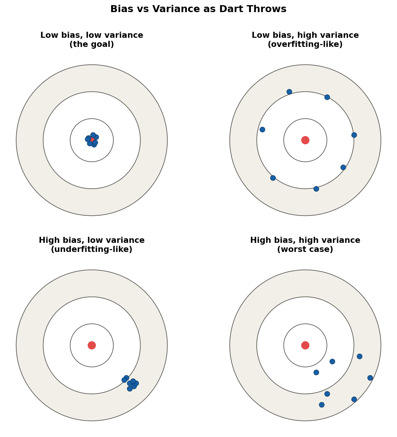
Before the formulas, here’s the intuition almost everyone reaches for when learning bias and variance for the first time: picture throwing darts at a dartboard, where the bullseye represents the true underlying pattern your model is trying to hit, and each dart is one prediction your model makes.
- Bias is how far off-center your darts land, on average. If every dart consistently lands in roughly the same spot away from the bullseye, that’s high bias — your model is systematically wrong in the same direction every time, because it’s too simple to represent the true pattern.
- Variance is how spread out your darts are from each other. If your darts scatter all over the board — sometimes near the bullseye, sometimes far, in different directions each time you throw — that’s high variance, because your model is too sensitive to the specific quirks of whatever training data it happened to see.
Four dartboards showing every combination of bias and variance: tightly clustered on target for low bias and low variance, scattered but centered for low bias and high variance, tightly clustered but off-target for high bias and low variance, and scattered and off-target for high bias and high variance
Top-left is the goal — every throw lands near the bullseye, consistently. Top-right shows low bias but high variance: the throws average out to the bullseye, but any individual throw could land almost anywhere — this is what overfitting looks like, since the model does fine “on average” across many retrainings but is wildly unstable for any one specific training set. Bottom-left shows high bias but low variance: the throws are tightly clustered together, so the model is stable and consistent, but consistently wrong — this is what underfitting looks like. Bottom-right, high bias and high variance, is the worst of both worlds: inconsistent AND consistently off-target.
Why this maps cleanly onto model training: each “dart throw” corresponds to training your model on one particular sample of data and then making a prediction. If you retrained your model on 100 different (but similarly-collected) datasets and plotted where each retrained model’s prediction landed, the pattern those 100 dots make on the board is precisely what bias and variance describe.
4.3 Bias and Variance in Everyday Model Behavior
It helps to ground this in what you’d actually observe while training a model, not just the dartboard picture:
| Signal you’d notice | What’s happening | Bias or variance? |
|---|---|---|
| Model performs poorly even on training data | It can’t even fit the data it’s seen — too rigid | High bias |
| Model performs great on training data, poorly on new data | It memorized quirks specific to the training set | High variance |
| Retraining on a slightly different sample barely changes predictions | The model is stable and consistent | Low variance |
| Retraining on a slightly different sample gives a very different model | The model is unstable, overly sensitive to its specific sample | High variance |
| The model’s mistakes always lean the same direction, regardless of which training sample was used | The model has a fixed, structural blind spot | High bias |
4.4 Step 2: Defining Bias Formally
Bias measures how far off, on average, your model’s predictions are from the true underlying pattern, due to the model being too simple to capture it.
Why this makes sense in plain words: if you trained your model on many different random samples of training data, and every single time it consistently misses the true pattern in the same systematic way (e.g., a straight line always underestimating salary at high experience levels because the true relationship curves), that consistent, repeated miss is bias. High bias is the mathematical fingerprint of underfitting — the model is too rigid to represent the truth, no matter how much or which training data you give it.
4.5 Step 3: Defining Variance
Variance measures how much your model’s predictions swing around if you retrained it on a slightly different sample of training data.
Why this makes sense in plain words: if your model is so flexible that it fits every quirk of whatever specific training data it happens to see, then training it on a slightly different dataset (even one drawn from the exact same true underlying pattern) would produce a very different fitted curve each time. That instability — a model whose output depends heavily on the exact noise in its specific training sample — is variance. High variance is the mathematical fingerprint of overfitting.
4.6 Step 4: The Tradeoff
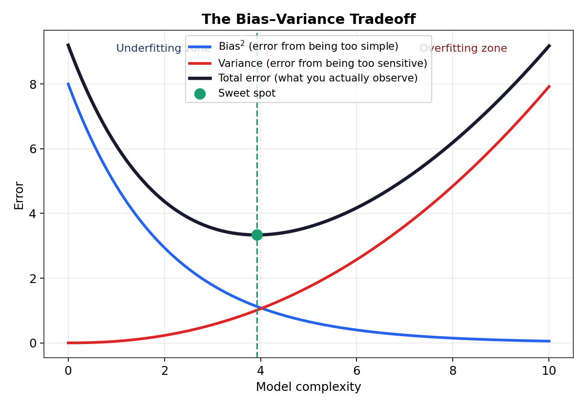
Critically, bias and variance pull in opposite directions as model complexity changes:
- Simple models (like a straight line) → high bias, low variance. They’re consistently wrong in the same way, but stable — retraining on a new sample barely changes the fitted line.
- Complex models (like a high-degree polynomial or a huge neural network) → low bias, high variance. They can represent the true pattern well in principle, but they’re unstable — small changes in training data cause big swings in the fitted curve.
4.7 Geometric Interpretation
A line chart showing bias squared decreasing, variance increasing, and total error forming a U-shape as model complexity increases, with a green marker showing the optimal sweet spot
As model complexity increases (moving right), bias (blue) steadily drops — a more flexible model can represent the true pattern more closely. But variance (red) climbs — that same flexibility makes the model increasingly sensitive to noise in whatever specific training data it sees. The total error (black) is their sum, forming a U-shape. The green “sweet spot” is the complexity level that minimizes total error — not the simplest model (underfitting, left zone) and not the most complex model (overfitting, right zone), but the balance point in between.
4.8 Detecting Overfitting Through Training
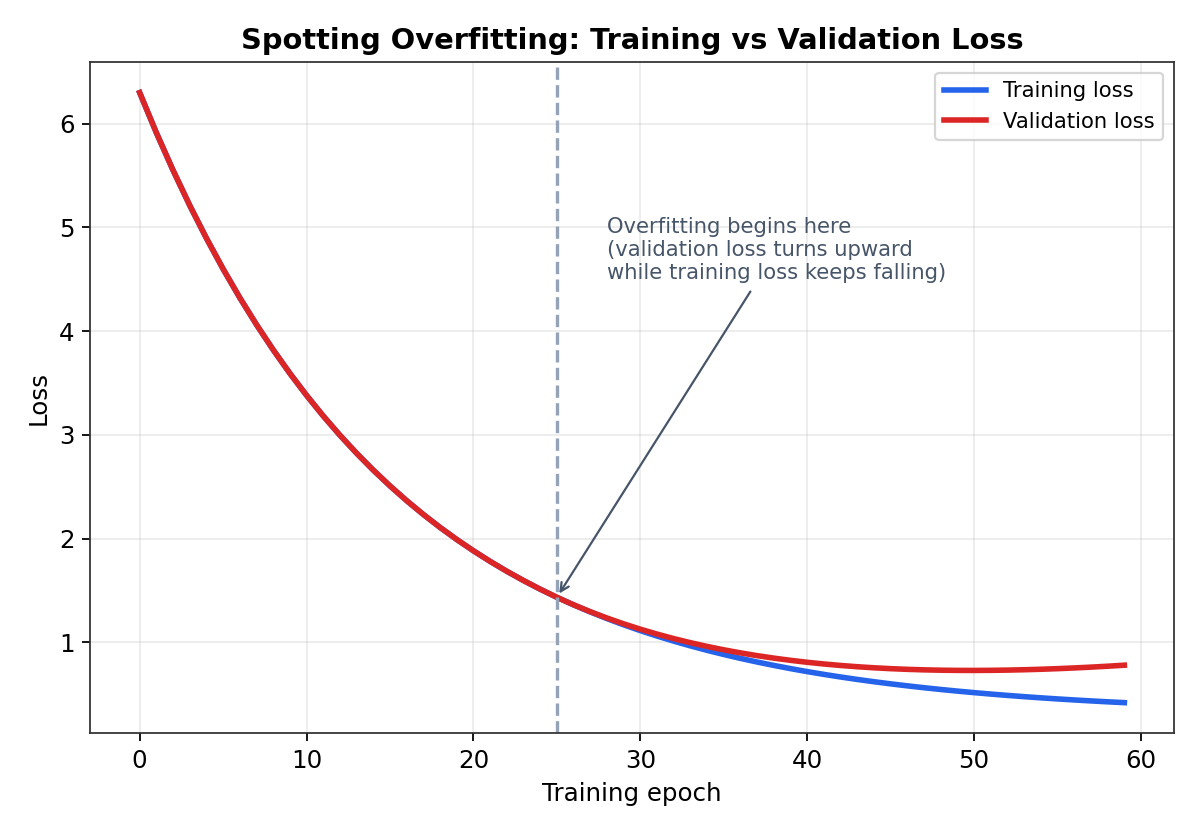
Beyond the bias-variance curve, overfitting can be spotted directly during the training process itself, by watching training loss and validation loss (using the cost function ideas from your earlier notes) across training iterations/epochs:
A line chart showing training loss steadily decreasing over epochs while validation loss decreases initially then turns upward, marking where overfitting begins
Early in training, both training loss (blue) and validation loss (red) fall together — the model is learning genuine, generalizable patterns. Past a certain point, training loss keeps falling (the model is still improving on data it has already seen), but validation loss starts climbing back up — the model has begun memorizing training-specific noise rather than learning anything that generalizes. This crossover point is exactly when overfitting begins, and it’s the signal used by a technique called early stopping, which halts training right around here rather than letting it continue.
5. Types / Variants — Ways to Prevent Overfitting
Overfitting isn’t just a diagnosis — there’s a well-established toolbox of countermeasures, each tackling the problem from a different angle.
- Regularization is like a teacher penalizing an exam answer for being needlessly convoluted, even if it happens to be technically correct — it discourages the model from relying too heavily on any single input feature.
- Cross-validation is like a rehearsal exam under slightly different conditions each time, so you catch a “memorizer” before the real exam, rather than after.
- Early stopping is like a coach pulling a runner off the track the moment their pace starts getting worse, rather than letting them run themselves into exhaustion.
- Dropout (specific to neural networks) is like randomly blindfolding a different subset of students during every practice round, so no single student becomes the “designated memorizer” the group secretly relies on.
- More training data is like giving the memorizing student (Student B from the Introduction) so many varied practice questions that memorizing individual answers stops being a workable shortcut — genuine understanding becomes the only strategy left.
| Technique | How it works | Best suited for | Analogy |
|---|---|---|---|
| Regularization (L1/L2) | Adds a penalty term to the cost function that discourages excessively large parameter values | Regression models, including SLR-style linear models | Docking marks for an overly convoluted exam answer |
| Cross-validation | Repeatedly splits data into different train/test partitions to check consistency of performance | Any model, especially with limited data | Rehearsal exams under varied conditions |
| Early stopping | Halts training once validation loss stops improving, even if training loss is still falling | Iterative training methods like gradient descent | Pulling a runner off the track before they overexert |
| Dropout | Randomly disables a fraction of neurons during each training step | Deep neural networks | Randomly blindfolding different students each round |
| More / better training data | Increases the diversity of examples the model sees, making memorization impractical | Any model, when more labeled data is available | Enough varied practice questions that memorizing stops working |
6. Limitations and Trade-offs
6.1 Underfitting: A Concrete Failure Case
Worked example: Suppose you use Simple Linear Regression (a single straight line) to predict salary from experience, but the true relationship curves and tapers off at higher experience. On your training data, the straight line will show a consistently high MSE — not because of any single bad data point, but because a straight line simply cannot bend to match the true curved pattern, no matter how the line’s slope and intercept are adjusted. This is the geometric-squares problem from your SLR notes, except here the issue isn’t noise in individual points — it’s that the model’s entire shape is fundamentally wrong for the task.
How it’s addressed: increasing model complexity — for instance, using polynomial regression (mentioned in your SLR notes’ Types section) or a more flexible model — allows the fitted curve to actually bend and match the true underlying pattern.
6.2 Overfitting: A Concrete Failure Case
Worked example: Now push in the opposite direction — fit a very high-degree polynomial (or an overly large neural network) to the same salary dataset. As shown in the rightmost panel of the fit-comparison diagram in section 3.2, the curve will wiggle wildly to pass almost exactly through every single training point — including points that are just off due to random noise (like one employee negotiating an unusually high salary for reasons unrelated to experience). On the training set, MSE will look almost perfect. But feed this model a new employee’s experience value, and its wild wiggling can produce a wildly inaccurate salary prediction, especially between training points or beyond the training range — the model has learned the noise, not the signal.
How it’s addressed: exactly the toolbox from section 5 — regularization, cross-validation, early stopping, dropout, or more training data — each of which constrains the model’s tendency to chase every quirk of its specific training sample.
6.3 The Deeper Trade-off: You Can’t Fully Escape It
Even with every countermeasure applied, the bias-variance tradeoff from section 4.4 doesn’t disappear — it’s a fundamental mathematical relationship, not a bug to be patched away entirely. Reducing bias by increasing model complexity will always tend to increase variance somewhat, and vice versa. The goal of all these techniques isn’t to eliminate the tradeoff, but to find and stay near the “sweet spot” from section 4.5 as reliably as possible.
7. Connecting to What You Already Know
The MSE, MAE, RMSE, and R² connection: these are exactly the metrics you use to measure training error and test error when diagnosing overfitting/underfitting, as shown in the table in section 3.3. A large gap between training MSE and test MSE, or a training R² much higher than a test R², is a direct numerical signal of overfitting.
The Cost Function and Convergence connection: early stopping is literally applying a modified convergence rule from your Convergence notes — instead of stopping when the training cost function stops improving, you stop when the validation cost stops improving (or starts getting worse), even if training cost is still falling.
The SLR and polynomial regression connection: Simple Linear Regression, being a single straight line, is inherently a low-complexity model — prone to underfitting on genuinely curved relationships, but comfortably safe from overfitting precisely because it has so few parameters () to “memorize” noise with. This is exactly why your SLR notes’ Types section introduced polynomial regression as the fix for underfitting on curved data — but as this section’s math shows, cranking that polynomial degree up too far swings the pendulum straight into overfitting instead.
The perceptron and deep learning connection: a single perceptron, like SLR, has very few parameters and tends toward underfitting on complex problems. Deep neural networks, by contrast, often have millions of parameters — far more expressive power, which is exactly why techniques like dropout were invented specifically for them, as mentioned in the History section: the same flexibility that lets deep networks learn extraordinarily complex patterns also makes them prone to memorizing training data unless deliberately restrained.
The machine learning types connection: overfitting and underfitting apply across both regression (like SLR, predicting salary) and classification problems (like logistic regression) — the same bias-variance tradeoff and training-vs-test-error diagnostic apply regardless of which type of supervised learning task you’re solving.
8. Quick Recap Table
| Concept | Meaning |
|---|---|
| Underfitting | Model too simple to capture the real pattern; poor performance on both training and test data |
| Overfitting | Model too complex; memorizes training data (including noise), performing well on training data but poorly on test data |
| Generalization | A model’s ability to perform well on new, unseen data |
| Bias | Systematic error from a model being too simple to represent the true pattern |
| Variance | Instability in a model’s predictions caused by excessive sensitivity to the specific training data used |
| Dartboard analogy | Bias = how far off-center your throws land on average; variance = how spread out your throws are from each other |
| Bias-variance tradeoff | The fundamental relationship where reducing bias (via more complexity) tends to increase variance, and vice versa |
| Training error | How well a model performs on the data it was trained on |
| Test / Validation error | How well a model performs on new, unseen data |
| Regularization | Adding a penalty to the cost function to discourage excessive model complexity |
| Cross-validation | Testing model performance across multiple different train/test data splits |
| Early stopping | Halting training once validation performance stops improving, even if training performance is still improving |
| Dropout | Randomly disabling neurons during neural network training to prevent over-reliance on specific patterns |
| Occam’s Razor | The principle that, among equally valid explanations, the simplest one is generally preferable |
9. Key Takeaway
Overfitting and underfitting are two opposite failure modes of the same underlying challenge: building a model that captures the real pattern in your data without being distracted by its noise. Underfitting happens when a model is too rigid to learn the true relationship, showing up as high error on both training and test data; overfitting happens when a model is too flexible, memorizing training data (including its randomness) so well that it fails to generalize to anything new. The bias-variance tradeoff explains mathematically why you can’t simply maximize model complexity to solve everything — and the practical toolbox of regularization, cross-validation, early stopping, dropout, and more training data all exist to help you land as close as possible to the sweet spot between these two extremes, whether you’re fitting a simple line like SLR or training a deep neural network with millions of parameters.