Multiple Linear Regression
1. Introduction
Suppose you’re trying to guess the price of a house before it’s listed. If you only knew its size, you could make a rough guess — bigger house, higher price. But you’d be wrong a lot. Two houses of the same size can sell for very different prices depending on the number of bedrooms, the age of the house, and how good the neighborhood is.
A single input isn’t enough. You want to combine several pieces of information at once and let each one pull the prediction up or down by the right amount. That’s exactly the problem Multiple Linear Regression (MLR) solves.
Formal definition: Multiple Linear Regression is a method that predicts one dependent variable (the thing you want to know — here, price) using two or more independent variables (the things you already know — size, bedrooms, age), assuming the relationship between them is a straight-line (linear) one: each input contributes a fixed amount per unit, and the contributions just add up.
If you’ve heard of Simple Linear Regression (one input, one output, a straight line through a scatter plot), MLR is the natural extension: same idea, more inputs.
2. History
The story of MLR starts not with houses, but with planets.
In the early 1800s, astronomers were trying to predict the orbits of comets and asteroids from telescope measurements. The problem was that every measurement had a small amount of error — the telescope, the observer, the atmosphere, all introduced noise. Given several noisy, slightly-inconsistent observations, how do you find the single best orbit that explains them all?
In 1805, the French mathematician Adrien-Marie Legendre published a technique called the method of least squares — choose the curve that minimizes the total squared distance between the predicted and observed values. Shortly after, Carl Friedrich Gauss claimed he had been using the same method privately since 1795, when he used it to correctly predict the position of the dwarf planet Ceres after it had been lost from view. Their priority dispute is famous in the history of math, but the important part is this: least squares was born out of a very practical need to fit a line (or curve) through noisy data — which is precisely what regression still does today.
At this stage, though, the method was mostly used with one predictor at a time. The real shift came later in the 19th century with Sir Francis Galton, a scientist studying how children’s heights related to their parents’ heights. He noticed that unusually tall parents tended to have children who were tall, but usually not as tall — their heights “regressed” back toward the average. He called this phenomenon regression toward the mean, and the name stuck to the whole family of techniques, even though modern regression is about much more than this one observation.
Around the same time, statisticians realized that most real outcomes don’t depend on just one cause. A crop’s yield depends on rainfall and fertilizer and temperature, not any single one of them. Karl Pearson and later Ronald Fisher, working in the early 1900s, formalized the mathematics of correlation and regression with multiple variables, expressing everything in terms of matrix algebra — which made it possible, at least in principle, to fit a line using any number of inputs at once.
The “in principle” was the catch: solving these matrix equations by hand for more than two or three variables was brutally tedious. It wasn’t until digital computers became available in the mid-20th century that Multiple Linear Regression became a practical, everyday tool — first in statistics and economics, and later, as computing kept getting cheaper, as one of the very first algorithms taught in machine learning, because it’s simple, fast, and a natural stepping stone toward more complex models like neural networks.
3. Core Concepts
3.1 The Building Blocks
| Term | Plain-English Meaning |
|---|---|
| Dependent variable (target / label) | The thing you’re trying to predict. Usually written . |
| Independent variable (feature / predictor) | An input you use to make the prediction. Usually written . |
| Coefficient (weight) | A number that says how much a feature pulls the prediction up or down per unit. |
| Intercept (bias) | The baseline prediction when all features are zero. |
3.2 From One Feature to Many
Simple Linear Regression (one feature):
This draws a single straight line through a 2D scatter plot of vs .
Multiple Linear Regression (many features) simply extends this pattern — one more term per feature:
Nothing new conceptually happens when you go from 1 feature to 10 — you’re just adding more “” terms before summing them up.
| Simple Linear Regression | Multiple Linear Regression | |
|---|---|---|
| Number of features | 1 | 2 or more |
| Shape of the model | A straight line | A flat plane (2 features) or a “hyperplane” (3+ features) |
| Equation | ||
| Example use case | Predict price from size alone | Predict price from size, bedrooms, age, location |
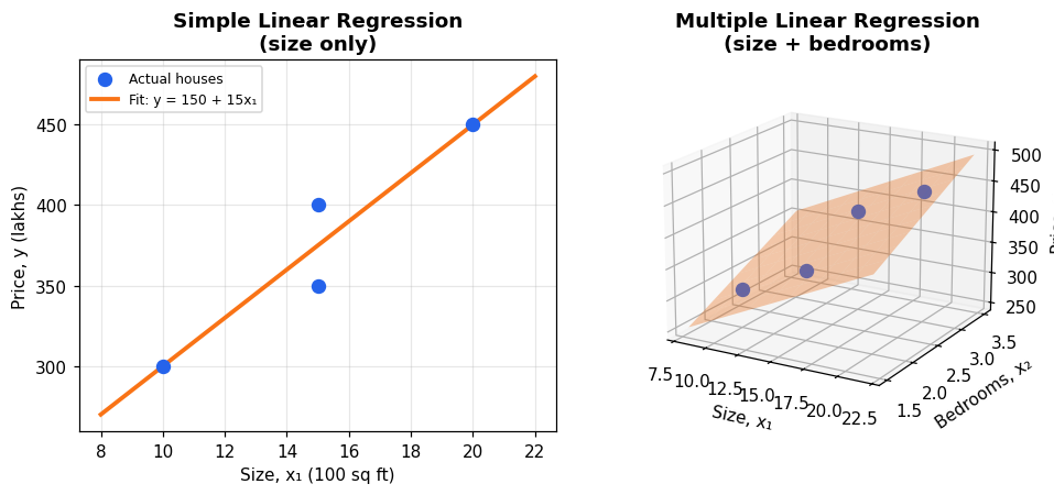
Simple regression (size only) vs multiple regression (size + bedrooms) on the same houses
3.3 The Geometric Picture
With 1 feature, you’re fitting a line through points on a 2D graph (x, y).
With 2 features, you’re fitting a flat plane through points floating in 3D space (x1, x2, y):
        y (price)
        |
        |        *
        |     *
        |   ______________  <- the fitted plane
        | *
        |________________________ x1 (size)
       /
      / x2 (bedrooms)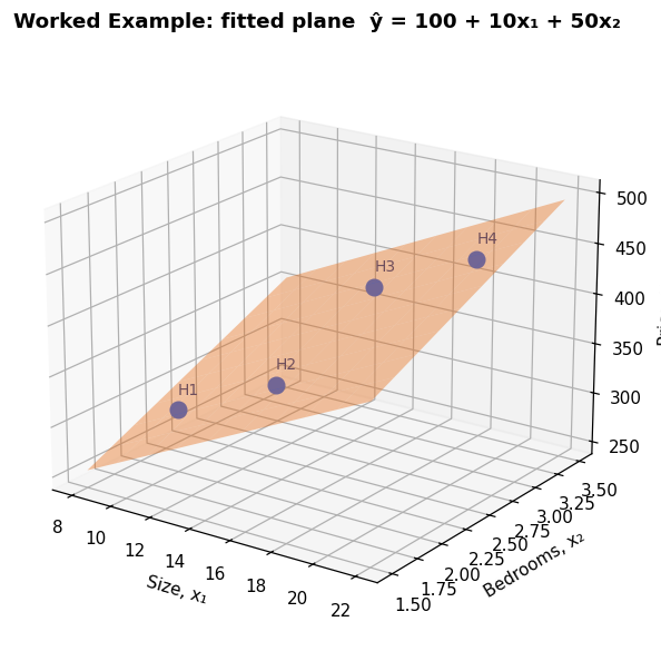
The four houses plotted in 3D with the fitted regression plane
With 3 or more features, you can no longer draw it, but the math works exactly the same way — statisticians call this generalized flat surface a hyperplane. “Hyper” just means “in more than 3 dimensions, which we can’t visualize, but can still compute.”
3.4 The Assumptions Behind MLR
MLR isn’t magic — it works well only when certain conditions roughly hold. These are the classic assumptions:
| Assumption | Plain-English Meaning |
|---|---|
| Linearity | The true relationship really is roughly a straight-line combination of the features, not curved. |
| Independence of errors | One prediction’s mistake doesn’t influence another’s (e.g., no hidden time pattern). |
| Homoscedasticity | The size of typical prediction error stays roughly constant across the range of inputs, instead of growing for larger values. |
| Normality of residuals | The leftover errors (actual − predicted) are roughly bell-curve shaped, useful mainly for statistical significance testing. |
| No severe multicollinearity | The features shouldn’t be near-duplicates of each other (more on why in Section 6). |
You don’t need to memorize these — just know that when a MLR model behaves strangely, one of these assumptions being violated is usually the reason.
4. The Math, Built Up Slowly
4.1 Symbol Table
| Symbol | Meaning |
|---|---|
| The actual observed value of the target (e.g., real price of a house) | |
| (“y-hat”) | The model’s predicted value |
| The input features | |
| The intercept (baseline prediction) | |
| The coefficients (weights) for each feature | |
| (“beta”) | Shorthand vector containing all coefficients, |
| A matrix holding all the feature values for every data point | |
| A vector holding all the actual target values | |
| Number of data points (rows) | |
| Number of features (not counting the intercept) | |
| (“epsilon”) | The error — the gap between what the model predicts and reality |
4.2 One Feature, Then Many
Start with one feature:
Add a second:
Generalize to features:
This is really just a dot product plus a constant. Quick refresher: the dot product of two lists of numbers means “multiply matching positions together, then add up the results.” So . The whole regression equation is just “dot product of weights and features, then add the intercept.”
4.3 Packing Everything Into Matrices
Writing this equation out separately for every row of data gets repetitive fast. Instead, statisticians stack all the data into a matrix (adding a column of 1’s so the intercept fits the same pattern as the other weights) and all the answers into a vector :
This single line represents every row of your dataset at once: “the actual values equal the matrix of features times the weight vector, plus whatever error is left over.”
4.4 How Do We Choose the Best Weights?
We want the that makes the predictions as close as possible to the actual values, across all rows at once. “Close” is measured using the Sum of Squared Errors (SSE):
Why squared? Two reasons: (1) it turns negative errors (predicted too low) and positive errors (predicted too high) into equally “bad” positive numbers, so they don’t cancel out, and (2) it punishes big mistakes much more than small ones — being off by 10 is worse than being off by 1, ten times over even before squaring, and 100 times worse after squaring.
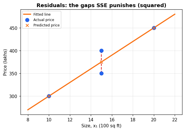
Residuals: the vertical gaps between actual and predicted price that SSE squares and sums
4.5 The Normal Equation
Calculus tells us that a smooth curve is at its lowest point exactly where its slope is zero. The “slope” here is with respect to each coefficient — so finding the best means solving the whole system of equations where every one of those slopes hits zero at once. Doing that algebra (we won’t derive it line-by-line here, but it’s a standard calculus result) for all coefficients simultaneously produces this closed-form formula, called the normal equation:
Piece by piece:
- means the transpose of — flip its rows and columns.
- multiplies the transposed matrix by itself — this produces a small square matrix summarizing how every feature relates to every other feature (including itself).
- is the matrix inverse — the matrix equivalent of “dividing by a number.” Just like , a matrix times its inverse gives the identity matrix (matrix version of “1”).
- summarizes how each feature relates to the actual target values.
- Multiplying it all together gives you the exact set of weights that minimizes the SSE.
4.6 Plugging In Real Numbers
Here’s a tiny made-up dataset, predicting house price (in lakhs) from size (in units of 100 sq ft) and bedrooms:
| House | Size () | Bedrooms () | Price () |
|---|---|---|---|
| 1 | 10 | 2 | 300 |
| 2 | 15 | 2 | 350 |
| 3 | 15 | 3 | 400 |
| 4 | 20 | 3 | 450 |
Adding a column of 1’s for the intercept, our matrix and vector are:
Computing (each entry is a sum of products across the 4 rows):
Computing :
Solving gives:
You can hand-verify this without inverting anything — just plug these numbers into the three equations that represents, and check both sides match:
- Row 1: ✓ (matches row 1)
- Row 2: ✓
- Row 3: ✓
All three check out, so is confirmed correct. Now plug it back into the original equation to double check the predictions match the actual prices exactly:
- House 1: ✓
- House 2: ✓
- House 3: ✓
- House 4: ✓
Every prediction matches perfectly — because this toy data was built from an exact linear rule with no noise. Real data will almost never fit this perfectly; there will usually be leftover error () even with the best possible .
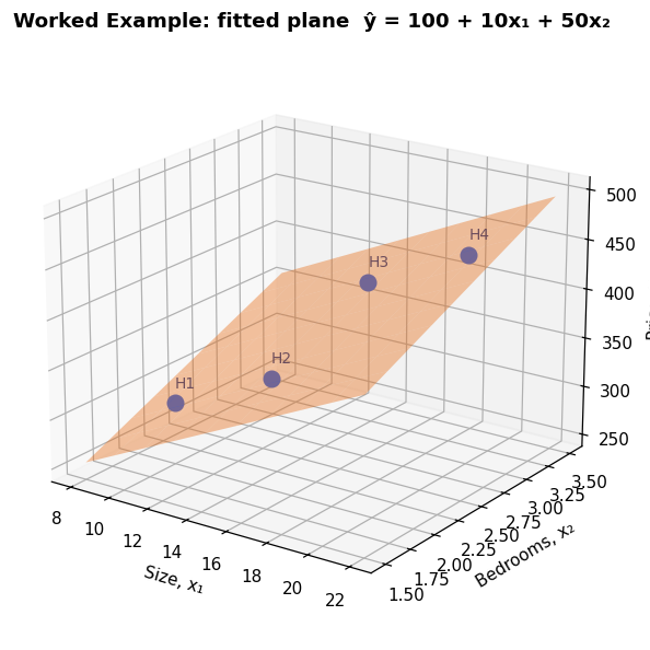
The exact fitted plane from the worked example|361
5. What The Math Is Actually Doing
Underneath all the matrix notation, the normal equation is just doing something very intuitive: it’s asking “for every combination of weights I could choose, how far off would my total predictions be, squared and added up — and which single combination makes that total as small as possible?” The matrix algebra is a shortcut that jumps straight to that best combination instead of guessing-and-checking millions of possibilities. In the house example, the model effectively learned that every extra “100 sq ft unit” of size is worth 10 lakhs, every extra bedroom is worth 50 lakhs, and even a house with zero size and zero bedrooms (a nonsensical but mathematically necessary baseline) would start at 100 lakhs — and it found those exact numbers by minimizing total squared error across every house at once, not by looking at any single house in isolation.
6. Types / Variants
Plain Multiple Linear Regression is the starting point, but it has well-known cousins built to fix specific weaknesses:
| Variant | Analogy | What It Changes |
|---|---|---|
| Ordinary MLR | A straight ruler laid across your data points | Minimizes SSE only, no extra constraints |
| Polynomial Regression | Bending that ruler into a curve | Adds squared/cubed versions of features () — still “linear” in the weights, just curved in the features |
| Ridge Regression | A ruler with a rubber band pulling all weights gently toward zero | Adds a penalty for large coefficients (L2 penalty) — reduces instability from multicollinearity |
| Lasso Regression | A ruler that will happily snap some weights to exactly zero | Adds a penalty that can eliminate less useful features entirely (L1 penalty) — doubles as feature selection |
| Elastic Net | A ruler with both a rubber band and a snapping mechanism | Combines Ridge’s and Lasso’s penalties together |
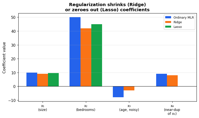
Ridge shrinks coefficients toward zero; Lasso can zero them out entirely
7. Limitations — Worked Examples
7.1 Multicollinearity: When Features Copy Each Other
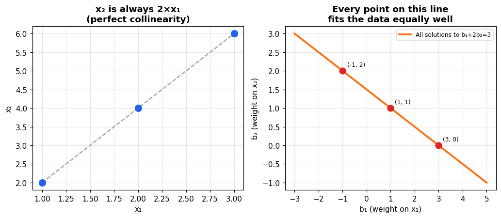
Left: two perfectly correlated features. Right: infinitely many (b1, b2) fit equally well
Suppose two features are near-duplicates. Take this tiny dataset where is always exactly :
| Row | |||
|---|---|---|---|
| 1 | 1 | 2 | 3 |
| 2 | 2 | 4 | 6 |
| 3 | 3 | 6 | 9 |
The true rule could be , or equally, , or a mix like (check: ✓, ✓, ✓). All of these fit the data perfectly — meaning there is no single “correct” answer for how much credit belongs to versus . The math has infinitely many valid solutions, and small amounts of noise can flip the coefficients from strongly positive to strongly negative between two runs of the same model on slightly different data. This is what multicollinearity does in practice: the model’s predictions stay accurate, but the individual coefficients become meaningless and unstable — dangerous if you’re trying to interpret “how much does bedroom count matter,” rather than just predict price.
Fix: Ridge regression’s penalty discourages any one coefficient from growing huge to compensate for another, which stabilizes this exact situation. Alternatively, you can just drop one of the redundant features.
7.2 Overfitting: Too Many Features, Too Little Data
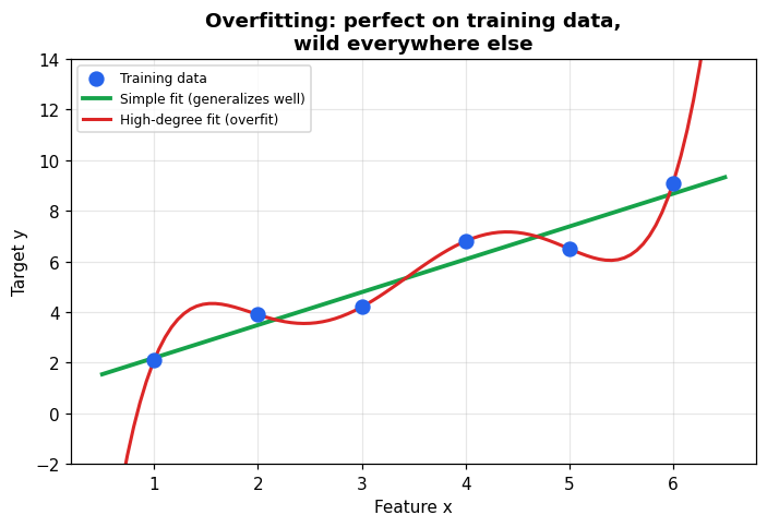
A simple fit that generalizes vs a high-degree fit that overfits the training points
If you have, say, 3 data points but use 3 features (plus an intercept — 4 total parameters), the model has enough flexibility to fit those 3 points exactly, even if the points were pure random noise with no real underlying pattern. It isn’t “learning” anything general — it’s just memorizing. On brand-new houses it hasn’t seen, its predictions can be wildly wrong despite a perfect fit on the training data.
Fix: Collect more data relative to the number of features, use regularization (Ridge/Lasso), or use fewer, more meaningful features.
7.3 Other Limits
- MLR assumes a straight-line relationship — if price actually rises steeply then plateaus, MLR will fit it poorly unless you add polynomial terms.
- A few extreme outliers can drag the whole fitted plane toward them, since squared error punishes big misses heavily.
- Extrapolating far outside the range of your training data (predicting the price of a 10,000 sq ft mansion when your data tops out at 2,000 sq ft) is unreliable — the straight-line relationship may not hold that far out.
8. Connecting This To The Bigger Picture
Even without having covered other topics yet in this chat, it’s worth knowing where MLR sits in the wider landscape you’re heading toward:
- A perceptron (the basic unit of a neural network, loosely inspired by a biological neuron) computes exactly the same weighted-sum-plus-bias formula as MLR — — and then usually passes it through an “activation function.” If you remove the activation function (or use the simplest possible one, the identity function), a single perceptron is Multiple Linear Regression.
- A neural network is, at its core, many of these weighted sums stacked and chained together with nonlinear activation functions in between, which is what lets it model curved, complex relationships that plain MLR cannot.
- The normal equation gives an exact, one-shot solution for MLR because the SSE cost function has a nice bowl shape (mathematically: it’s convex). Neural networks don’t have this luxury — their cost functions are far more complicated, so instead of solving directly, they use gradient descent, an iterative “take small steps downhill” method. Learning gradient descent next will make much more sense once you’ve seen the “downhill” shape MLR’s own cost function has.
In short: MLR is the simplest possible neural network, and the least squares problem it solves is the friendliest possible version of the optimization problem every deep learning model is ultimately trying to solve.
9. Quick Recap Table
| Concept | Meaning |
|---|---|
| Dependent variable () | What you’re predicting |
| Independent variable () | An input used to predict |
| Coefficient () | How much each feature moves the prediction |
| Intercept () | Baseline prediction when all features are 0 |
| matrix | All feature values for all rows, stacked together |
| vector | All actual target values |
| Sum of Squared Errors (SSE) | Total squared gap between predictions and reality |
| Normal equation | — the exact formula for the best-fit weights |
| Multicollinearity | Features that are near-duplicates of each other, causing unstable coefficients |
| Overfitting | Model memorizes training data instead of learning a general pattern |
| Ridge / Lasso / Elastic Net | Regularized versions of MLR that penalize large or unnecessary coefficients |
10. Key Takeaway
Multiple Linear Regression predicts an outcome by combining several inputs, each weighted by how much it matters, into one straight-line (or flat-plane, or hyperplane) equation — and it finds the single best set of weights by minimizing total squared prediction error across all the data at once, using the closed-form normal equation. It’s simple, interpretable, and exact when its assumptions hold, but it becomes shaky when features overlap with each other (multicollinearity) or when there isn’t enough data to support the number of features used (overfitting). Most importantly, it’s not just a standalone statistics tool — it’s the mathematical seed from which perceptrons, and eventually entire neural networks, grow.