Gradient Descent
1. Introduction
Imagine you’re hiking down a mountain in thick fog, at night, with only a small flashlight that lights up the ground right around your feet. You can’t see the valley below, you can’t see a map — all you can do is feel which direction the ground under your feet slopes downward, take one step that way, and repeat. Step by step, feeling and moving, you eventually reach the bottom of the valley, even though you never once saw the whole mountain.
This is almost exactly the situation a machine learning model is in when it “learns.”
A model has internal dials called parameters — for example, the slope and intercept of a line you’re fitting to data. When the model makes a prediction, we measure how wrong it is using a loss function (also called a cost function): a single number that is large when the model is doing badly and small when it’s doing well. “Training” a model just means searching for the parameter values that make this loss number as small as possible.
The problem is that this “loss landscape” can have thousands or millions of dimensions (one for every parameter in a real model), there is no map of it, and we can’t just eyeball where the lowest point is. Gradient Descent is the fog-and-flashlight strategy for finding it anyway: at your current position, feel the local slope, take a step in the downhill direction, and repeat until you stop making progress. It is arguably the single most important algorithm in all of machine learning and deep learning — nearly every model you will ever train, from simple linear regression to giant neural networks, is fitted to data using some version of this idea.
Formal definition: Gradient Descent is an iterative optimization algorithm that finds the input values which minimize a function, by repeatedly moving in the direction that decreases the function’s output the fastest — the direction opposite to the gradient (the local uphill direction).
2. History
The idea did not begin in machine learning at all — it began in 19th-century mathematics, over a hundred years before anyone used the phrase “machine learning.”
In 1847, the French mathematician Augustin-Louis Cauchy was wrestling with large systems of equations that had no clean, direct algebraic solution — the kind that show up when you’re trying to fit a curve through many astronomical observations at once. Cauchy proposed a simple, general strategy: at your current guess, compute the direction in which the function grows fastest, then move a small step in the opposite direction, and repeat. He called it the method of steepest descent, and it is the direct ancestor of every gradient descent variant used today.
For the next hundred years, the method stayed mostly inside numerical analysis and optimization theory, used by mathematicians and engineers to solve equations that could not be solved by hand. A key theoretical step came in 1951, when Herbert Robbins and Sutton Monro developed the theory of stochastic approximation — showing that you could still reliably converge toward a minimum even if, at every step, you only used a noisy or partial estimate of the true slope, rather than the exact one. This became the mathematical foundation for using randomly sampled data at each step, instead of the entire dataset.
The idea entered the world of learning machines in 1960, when Bernard Widrow and Ted Hoff introduced ADALINE (Adaptive Linear Neuron) and its training rule, the Delta Rule — an early artificial neuron trained by nudging its weights downhill along the error surface, essentially gradient descent applied to a single neuron. This ran in parallel with Frank Rosenblatt’s Perceptron (1958), which used a related but distinct update rule.
The real turning point for deep learning came in 1986, when David Rumelhart, Geoffrey Hinton, and Ronald Williams popularized backpropagation — a method for efficiently computing the gradient of the loss with respect to every weight in a multi-layer network, using the chain rule from calculus. Backpropagation did not replace gradient descent; it simply made gradient descent practical for deep, multi-layer networks by solving the “how do I even compute the slope for a weight buried three layers deep?” problem. This combination reignited interest in neural networks after a period of stagnation.
Through the 1990s and 2000s, as datasets grew too large to process all at once, Stochastic Gradient Descent (SGD) — using one or a few random examples per step, building directly on Robbins and Monro’s theory — became the practical default for large-scale learning. Finally, between 2011 and 2015, a wave of smarter variants arrived to handle the huge, complicated loss landscapes of deep learning: Adagrad (2011), RMSProp (2012), and Adam (2014), all of which are gradient descent at their core, but with extra bookkeeping to automatically adjust the step size as training proceeds. Adam in particular remains one of the most widely used optimizers in deep learning today.
3. Core Concepts
We’ll build this up piece by piece, from a single knob to many knobs at once.
3.1 What are we trying to minimize? The Loss Function
Suppose you’re building a model to predict something — a price, a score, a probability. The model will be wrong sometimes. The loss function (sometimes called cost function, written ) is a formula that turns “how wrong the model currently is” into a single number. Big number = bad predictions. Small number (ideally zero) = great predictions. Training a model is nothing more than searching for the parameter values that make as small as possible.
3.2 What is a Parameter?
A parameter is a dial the model can adjust to change its behavior. For a simple straight-line model (“predicted equals slope times plus intercept”), the parameters are (the slope) and (the intercept). Before training, we don’t know good values for them — we usually start with a guess (often 0) and let gradient descent improve it.
3.3 Slope: The One-Knob Building Block
If you have just one parameter, picture the loss function as a curve — a bowl shape, like the cross-section of a valley. At any point on that curve, the slope tells you two things: which direction is “uphill” (increasing) and how steep it is. If the slope is positive, the curve is going up as you move right, so you should move left to decrease . If the slope is negative, you should move right. This is the whole idea in miniature: always step in the direction opposite to the slope.
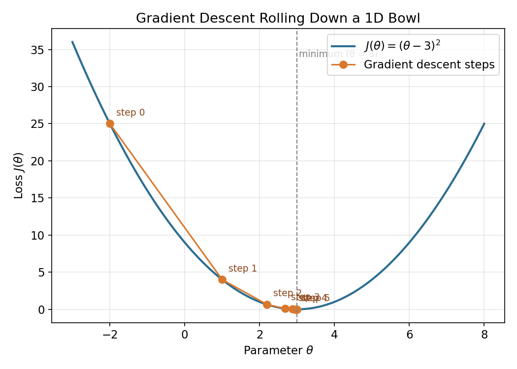
Gradient descent rolling down a 1D bowl-shaped loss curve, with labeled steps converging toward the minimum
3.4 From Slope to Gradient: Many Knobs at Once
Real models rarely have just one parameter — a simple linear regression already has two ( and ), and a neural network can have millions. When you have more than one parameter, “slope” generalizes to something called the gradient: instead of one number, it’s a list of numbers, one per parameter, where each number tells you the slope in that parameter’s direction only, holding all the others fixed. The gradient, as a whole, points in the direction of steepest increase of the loss — so, just like before, we move opposite to it to decrease the loss.
3.5 The Descent Step: Direction and Size
Every step of gradient descent has two ingredients:
| Ingredient | Question it answers | Where it comes from |
|---|---|---|
| Direction | Which way is downhill? | The negative gradient of the loss |
| Step size | How far do we move that way? | A number we choose, called the learning rate |
Take a step, recompute the slope at the new position (the ground looks different from here), take another step, and repeat. That loop — measure slope, step downhill, repeat — is gradient descent, in its entirety.
| Term | 1-parameter version | Many-parameter version |
|---|---|---|
| Local “which way is up” | slope (a single number) | gradient (a list of numbers, one per parameter) |
| Symbol | (“nabla J”) | |
| What we do with it | move opposite its sign | move opposite its direction |
4. The Math, Built Up Slowly
4.1 Symbol Table
| Symbol | Read as | Plain-English meaning |
|---|---|---|
| “theta” | A stand-in for “some parameter,” e.g. or | |
| “J of theta” | The loss function — how bad the model’s predictions are, as a function of the parameters | |
| “dJ by d-theta” | The derivative: how much changes for a tiny change in (the slope) | |
| “gradient of J” | The list of slopes, one per parameter, when there’s more than one | |
| “alpha” | The learning rate — how big a step to take | |
| “is updated to” | “Take the value on the right, and that becomes the new value on the left” | |
| “y hat” | The model’s prediction | |
| “y” | The true/actual value from the data | |
| “n” | Number of data points | |
| “sum over” | Add up a series of terms, one for each data point |
Quick prerequisite — what is a derivative? For a curve , the derivative at a point is the slope of the line that just touches the curve there (the tangent line). It answers: “if I nudge a tiny bit, how much and in which direction does move?” Positive derivative = increases as increases. Negative = decreases as increases.
4.2 Building the Update Rule, Piece by Piece
We want a rule that nudges to make smaller. Let’s build it one piece at a time instead of dropping the final formula on you.
Piece 1 — we need to know which way is uphill. That’s exactly what the derivative tells us.
Piece 2 — we want to move the opposite way. So we use , a minus sign flips uphill into downhill.
Piece 3 — we don’t want to leap wildly; we want a controlled step. So we scale that direction by a small positive number , the learning rate.
Piece 4 — apply that step to update our current guess. Old value plus the (scaled, flipped) slope gives the new value:
That’s it — that single line is gradient descent for one parameter. In plain English: “new guess = old guess, moved a small amount in the downhill direction.”
When there is more than one parameter, every symbol above just becomes a list (a vector, written in bold), and the derivative becomes the gradient:
Same sentence, same logic — it just updates every parameter at once, each by its own slope.
4.3 Worked Example 1 — A Single Parameter, By Hand
Let’s use the simplest possible loss curve: . This is a bowl whose lowest point (minimum) is obviously at , where — so we can check gradient descent’s work against an answer we already know.
Derivative: using the power rule (, a rule from calculus for differentiating a squared term), we get .
Start at (a bad guess, far from 3), with learning rate :
| Step | (current) | Gradient | Update: grad | New |
|---|---|---|---|---|
| 0 | ||||
| 1 | ||||
| 2 | ||||
| 3 | ||||
| 4 |
Notice the gradient’s magnitude shrinks as we approach — the ground gets flatter near the bottom of the bowl, so each step naturally gets smaller too, even with a fixed . This is exactly the path drawn in the diagram above.
4.4 Worked Example 2 — Two Parameters, Fitting a Line
Now the realistic case: fitting to actual data, where and must be tuned together.
Tiny dataset — hours studied () vs. score out of 10 ():
| (hours) | (score) |
|---|---|
| 1 | 2 |
| 2 | 4 |
| 3 | 5 |
Loss function — Mean Squared Error, the standard choice for this kind of problem:
Why squared? Squaring makes every error positive (so a error and a error don’t cancel out) and it punishes big mistakes much more than small ones — an error of 4 contributes 16, not just 4.
Working out the derivative with the chain rule (differentiating the outer square, then the inner linear term) gives two gradient formulas, one per parameter:
(The symbol, “partial,” just means “the derivative with respect to this one parameter, holding the others fixed” — it’s the multi-parameter version of .)
Step-by-step, starting from (the model knows nothing yet, so it predicts 0 for everything):
- Predictions:
- Errors ():
- Initial loss:
- Gradient for :
- Gradient for :
- Update, with :
- New predictions: — compare to the real : already close!
- New loss:
In a single step, the loss dropped from 15 to 0.234. That’s gradient descent, in full, on real (tiny) data.
4.5 What the Gradient Looks Like Geometrically
With two parameters, the loss surface becomes a 3D bowl, and it’s easiest to visualize by looking straight down at it — a contour plot, where each ring is a line of equal loss (like elevation lines on a topographic map). The gradient at any point always points directly toward the nearest higher ring (straight uphill, perpendicular to the contour line), so the negative gradient points straight downhill:
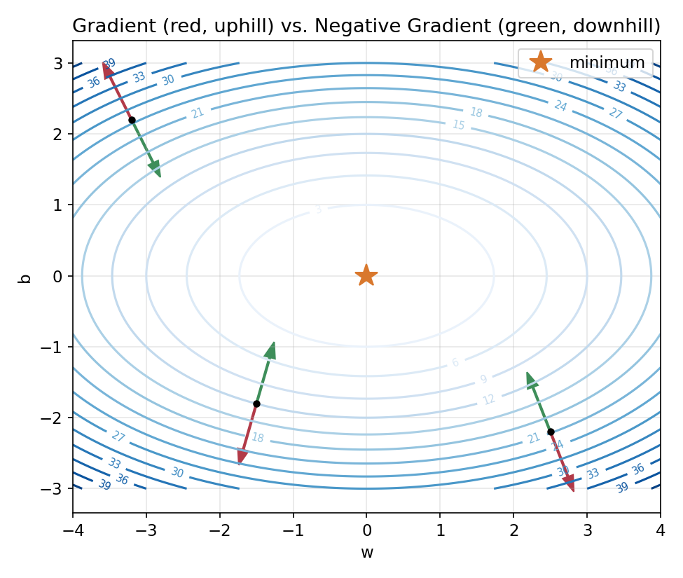
Contour plot showing the gradient direction (uphill, red) and negative gradient direction (downhill, green) at several points, both perpendicular to the contour lines, pointing toward and away from the minimum
5. What the Math Is Actually Doing
Zoom back out: none of this math is doing anything mysterious. Every single term in is answering one of the fog-hiker’s questions from the introduction. “Which way is downhill from here?” is answered by (or with many parameters) — the local slope, flipped to point downward. “How big a step should I take?” is answered by — too big and you might overshoot the valley floor and stumble up the other side; too small and you’ll be feeling your way down all night. And “:=” is simply “update your position and repeat” — feel, step, feel, step, until the slope is essentially flat and you know you’ve reached the bottom (or close enough to it).
6. Types / Variants
So far, our linear regression example used all the data to compute the gradient at every step. That’s one specific choice, called Batch Gradient Descent, and it’s just one of several variants — they all share the same core update rule, they only differ in how much data they look at before taking each step.
| Variant | Analogy | Data used per step | Speed per step | Path to the minimum |
|---|---|---|---|---|
| Batch GD | Tasting the whole pot of soup before adjusting the seasoning | All examples | Slow (recomputes everything) | Smooth, direct |
| Stochastic GD (SGD) | Tasting one random spoonful and adjusting immediately | 1 example | Very fast per step | Noisy, zig-zagging |
| Mini-batch GD | Tasting a few spoonfuls from different parts of the pot | A small batch (e.g. 32–256) | Fast, and GPU-friendly | Moderately noisy |
| Momentum | Remembering which way you’ve been walking, so you don’t stop dead at every bump | Any of the above, plus memory of past steps | Similar cost, fewer wasted steps | Smoother, faster through narrow valleys |
| Adaptive (Adagrad / RMSProp / Adam) | Automatically shortening your stride on steep ground and lengthening it on flat ground | Any of the above, plus per-parameter step-size history | Similar cost, extra bookkeeping | Self-adjusting, usually fastest in practice |
Batch GD gives the cleanest path because it always uses the true average gradient over all the data, while SGD’s path is noisy because a single example is often a poor stand-in for the whole dataset — but that noise is also what makes SGD dramatically cheaper per step, and is exactly the trade-off Robbins and Monro’s theory (Section 2) showed was still safe on average:
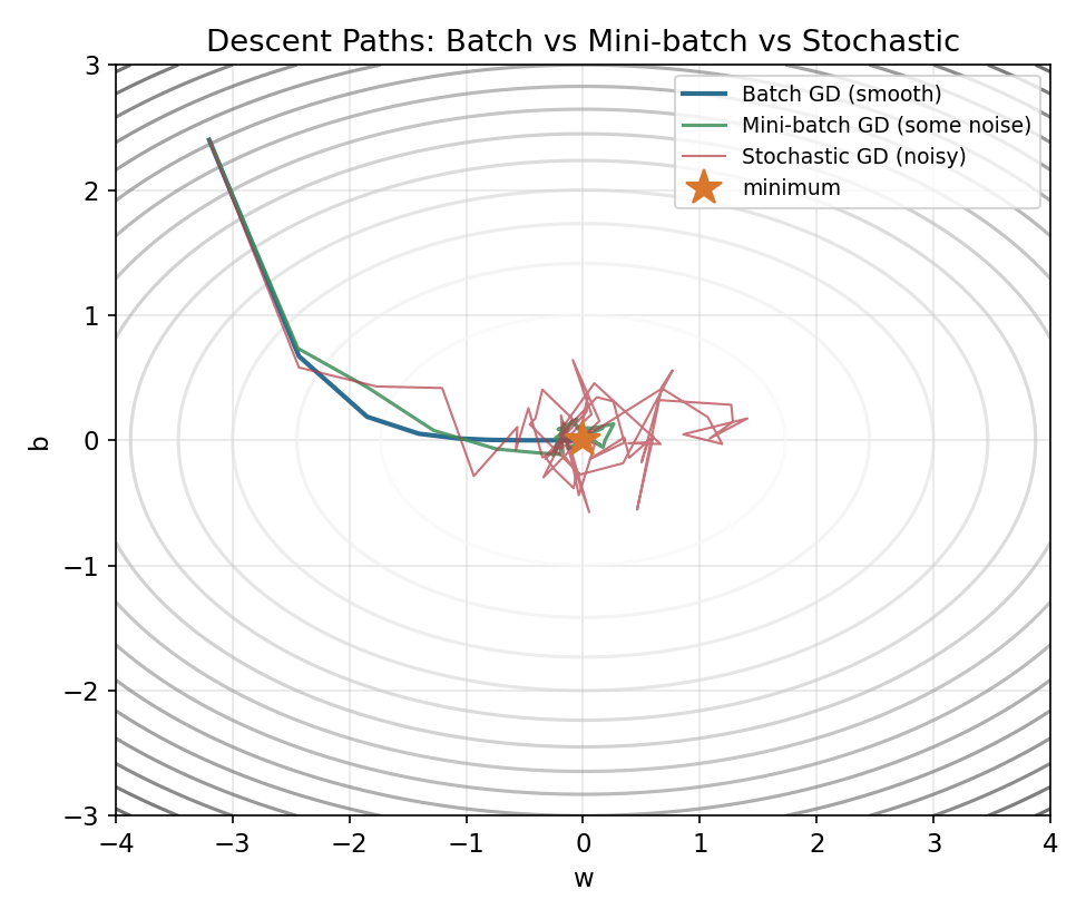
Contour plot comparing three descent paths from the same starting point: a smooth blue batch gradient descent path, a moderately noisy green mini-batch path, and a very noisy red stochastic gradient descent path, all converging to the same minimum
7. Limitations, Failure Modes, and Trade-offs
The learning rate is a double-edged sword. Reusing the 1D bowl from Section 4.3, watch what happens with three different values of , starting from the same point:
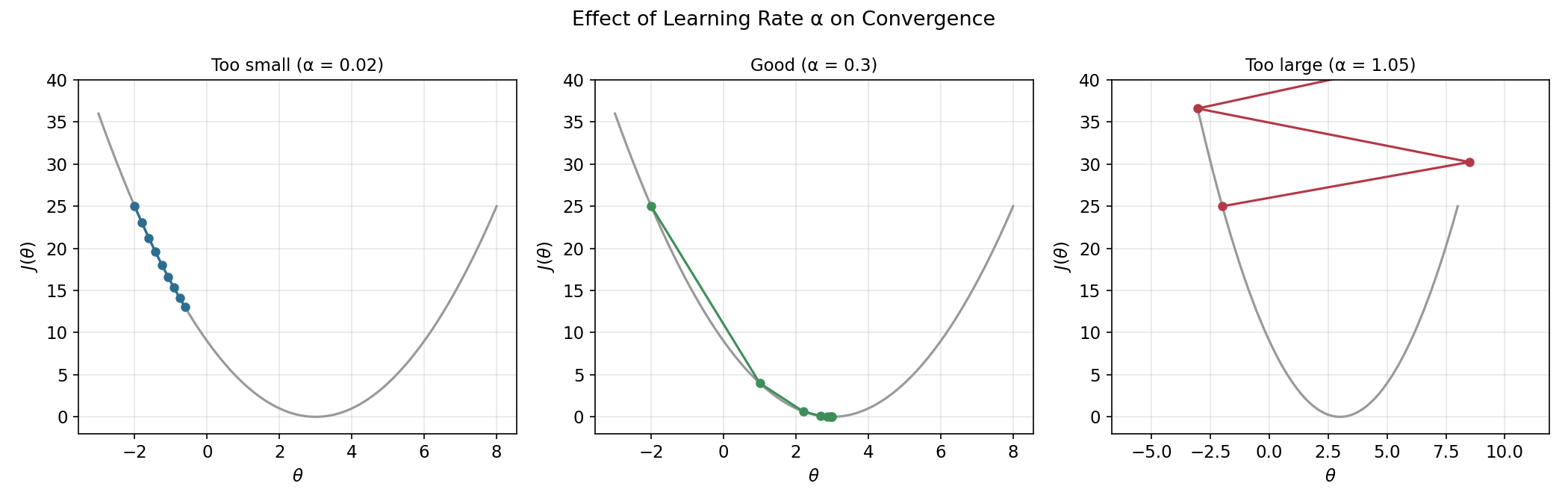
Three side-by-side plots comparing gradient descent with a learning rate that is too small (slow crawl), a good learning rate (smooth convergence), and too large (diverging, bouncing to ever-larger values)
With (too large) starting at : step 1 lands at — it didn’t just reach the minimum at 3, it overshot past it entirely. From there the next step overshoots even further in the other direction, and the parameter oscillates with growing amplitude instead of settling down. This is divergence, and it’s one of the most common beginner mistakes: picking a learning rate that feels “aggressive enough to train fast” but is actually too large for the shape of the loss surface. On the other end, a tiny never overshoots, but can take thousands of steps to travel a distance that a well-tuned covers in ten.
Not every loss surface is a nice, single bowl. Our examples were convex (bowl-shaped, with exactly one minimum, no other dips anywhere), which is why plain gradient descent always found it. Deep neural networks have loss surfaces with many bumps, dips, and flat stretches. Two specific failure modes:
- Local minima: a dip that looks like the bottom locally but isn’t the lowest point overall — the hiker reaches a small valley and, since the ground is flat all around, has no signal telling them to keep going.
- Saddle points / plateaus: flat or near-flat regions where the gradient is close to zero even though you’re nowhere near a good minimum — progress crawls to a near-halt.
How these are addressed in practice: momentum (Section 6) helps carry the optimizer through small dips and flat spots using “velocity” from previous steps, much like a rolling ball has enough momentum to coast over a small bump; adaptive methods like Adam automatically shrink the effective step size in steep, erratic directions and grow it in flat ones; learning rate schedules gradually shrink over training so early steps can be large and exploratory while later steps are small and precise; and good weight initialization and data normalization make the loss surface itself better-behaved to begin with, so there are fewer nasty bumps to navigate around.
8. Where This Fits Into Your Learning Journey
This is the first topic in your notes, so there’s no earlier material to link back to yet — but it’s worth being explicit about why this particular topic comes first: almost everything else you’ll learn in machine learning and deep learning is a variation on “define a loss, then use gradient descent to shrink it.” A short preview of what’s ahead, and how each connects directly back to what you learned today:
- Linear / logistic regression — exactly the two-parameter example from Section 4.4, just with a different loss function for logistic regression.
- The perceptron and ADALINE — the very first “learning machines” (Section 2), where a single artificial neuron’s weights are nudged using this same slope-following idea.
- Backpropagation — the technique that computes for every weight in a multi-layer neural network (potentially millions of parameters); once that gradient is known, the update step is the exact same line, , you already saw here.
- Deep learning training loops — every epoch of training any deep network is just: compute predictions, compute loss, compute gradients, take a gradient descent step (usually with Adam), repeat.
9. Quick Recap Table
| Concept | Meaning |
|---|---|
| Loss function | A single number measuring how wrong the model’s current predictions are |
| Parameter | A tunable dial in the model (e.g. a weight or bias) |
| Derivative | The slope of the loss curve — how much changes per tiny change in |
| Gradient | The list of slopes across all parameters at once; points in the steepest uphill direction |
| Learning rate | How big a step to take at each update |
| Update rule | — move opposite the slope, scaled by the learning rate |
| Convergence | When updates stop meaningfully changing — we’ve (approximately) reached a minimum |
| Batch GD | Uses the entire dataset for every gradient calculation |
| Stochastic GD (SGD) | Uses one random example per step |
| Mini-batch GD | Uses a small random subset per step |
| Momentum | Adds memory of past steps so descent doesn’t stall on bumps |
| Adaptive optimizers (Adam, etc.) | Automatically adjust the effective step size per parameter |
| Local minimum | A dip that looks like the bottom but isn’t the true lowest point |
| Divergence | When too-large a learning rate causes updates to overshoot and grow instead of shrink |
Key Takeaway
Gradient descent is nothing more than the fog-and-flashlight strategy, made mathematically precise: measure the local slope of how wrong you are, take a small step in the opposite direction, and repeat until the ground goes flat. Every extra idea in this document — batches, momentum, adaptive rates, even backpropagation itself — exists only to make that one simple loop work faster, more reliably, or on harder, bumpier terrain. Once this loop feels intuitive, you already understand the engine that trains nearly every machine learning and deep learning model that exists.