Epochs and Iterations
1. Introduction
Imagine you’re studying a deck of 23 flashcards for an exam. You could go through the entire deck once, put it down, then pick it up and go through it again — and again — several times over the course of your studying. Each full pass through the whole deck, front to back, is one unit of “practice.” But within a single pass, you’re also doing something smaller and more frequent: reviewing a handful of cards at a time before pausing, checking your answers, and adjusting how you think about the ones you got wrong.
Training a machine learning model works in exactly this two-layered way, and it’s easy to mix the two layers up if nobody ever draws the line between them clearly. Epochs and iterations are simply the names for those two layers: one epoch is one complete pass through the entire training dataset, and one iteration (also called a step) is one single update to the model’s parameters, based on just one chunk of that data. This distinction matters immensely in practice — the number of epochs and the size of the chunks (the batch size) directly control how long training takes, how noisy the learning process is, and whether the model ends up under-trained or over-trained.
Formal definitions, stated plainly:
- An iteration (or step) is one single execution of the gradient descent update rule — compute the gradient on one batch of data, then update the parameters once.
- An epoch is one complete pass through every example in the training dataset, made up of however many iterations it takes to cover all of it.
2. History
Unlike gradient descent itself, “epoch” and “iteration” aren’t really inventions with a single origin story — they’re bookkeeping terms that became necessary once training needed to be described precisely. But they do have a logical history worth walking through, because why the distinction had to be made is genuinely instructive.
In the earliest days of training simple learning machines, like Widrow and Hoff’s ADALINE in 1960, datasets were tiny — often just a handful of examples that comfortably fit in memory. It was completely normal to compute the gradient using every single example at once, take one update step, then repeat. In that world, there was no meaningful difference between “one pass through the data” and “one update step” — they were the same event, so nobody needed two separate words for it.
That started to change as neural network research grew through the 1980s, when backpropagation (Rumelhart, Hinton, and Williams, 1986 — see the Gradient Descent notes) made it practical to train multi-layer networks, and researchers began reporting how many times their networks had “swept through” the training set during learning. The word epoch entered the neural network vocabulary around this period, borrowed loosely from its everyday meaning of “a distinct period of time” — here, one full cycle through the data.
The real fork in the road came with the rise of big data in the 1990s and 2000s. As datasets grew from hundreds of examples to millions, computing the gradient over the entire dataset before taking even a single step became painfully slow, or outright impossible to fit in memory. The natural fix — already justified theoretically by Robbins and Monro’s 1951 stochastic approximation work — was to split the dataset into smaller chunks (mini-batches) and take an update step after each chunk, rather than waiting for the whole dataset. This is the moment “epoch” and “iteration” stopped being synonyms: an epoch could now contain many iterations, one for each mini-batch, and the two terms needed to be kept precisely separate to avoid confusion.
By the deep learning boom of the 2010s — accelerated by breakthroughs like AlexNet in 2012, trained on the million-plus-image ImageNet dataset — reporting both numbers became standard practice in every paper and every training log: how many epochs a model trained for, and how many iterations (or steps) that took given the chosen batch size. Around the same period, researchers formalized early stopping (with foundational work by Lutz Prechelt in the mid-1990s) — using the epoch-by-epoch validation performance, not individual iterations, as the natural checkpoint for deciding when a model has trained enough and should stop before it starts memorizing the training set.
3. Core Concepts
3.1 The Dataset
Everything here starts with the training dataset: the full collection of examples the model learns from. In our earlier Gradient Descent notes, our tiny “hours studied vs. score” dataset had just 3 examples. Real datasets can have millions. Let’s stay small and concrete: imagine a dataset with examples.
3.2 The Batch
Instead of using all examples for every single gradient calculation (as our earlier examples did, since was so small), we usually split the dataset into smaller chunks called batches. The batch size, written , is simply how many examples go into each chunk.
3.3 The Iteration (Step)
One iteration is: take one batch, run it through the model, compute the loss and its gradient on just that batch, and apply one gradient descent update. This is precisely the update rule from the Gradient Descent notes, , executed exactly once.
3.4 The Epoch
One epoch is complete once every example in the dataset has been used in exactly one batch — in other words, once you’ve marched through all the batches, one iteration at a time, and covered the whole dataset. If the dataset doesn’t split evenly into batches, the last batch of the epoch is simply smaller than the rest (more on this in Section 4).
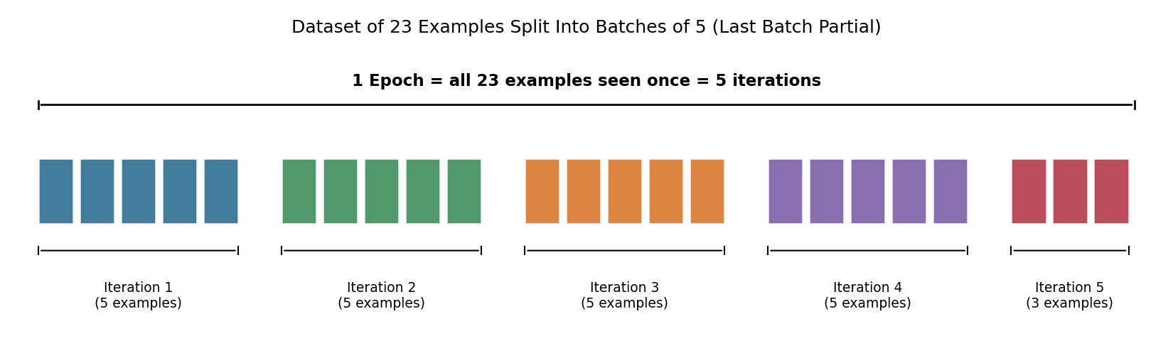
Schematic showing a dataset of 23 examples split into 5 batches of size 5, 5, 5, 5, and 3, each batch labeled as one iteration, with a bracket showing all 5 iterations together making up 1 epoch
3.5 Putting It Together — The Training Loop
Training a model is simply this structure, repeated: an outer loop over epochs, and an inner loop over iterations (batches) within each epoch.
for epoch in 1 ... E:                    # outer loop: repeat E times
    for batch in dataset's batches:      # inner loop: one pass through all data
        predictions = model(batch)
        loss = compute_loss(predictions, batch_targets)
        gradients = compute_gradients(loss)
        parameters = parameters - learning_rate * gradients   # one iteration
# <- one epoch complete here| Term | What it is | How many happen in one full training run |
|---|---|---|
| Example | One row of data | total |
| Batch | A chunk of examples processed together | batches per epoch |
| Iteration / step | One parameter update, using one batch | Same count as batches, per epoch |
| Epoch | One full pass through all examples | Chosen by you, e.g. times |
4. The Math, Built Up Slowly
4.1 Symbol Table
| Symbol | Read as | Plain-English meaning |
|---|---|---|
| “N” | Total number of examples in the training dataset | |
| “B” | Batch size — number of examples used per iteration | |
| “I” | Iterations per epoch — how many update steps it takes to cover the whole dataset once | |
| “E” | Number of epochs — how many times we sweep through the whole dataset | |
| “T” | Total iterations across the entire training run | |
| “ceiling of” | Round up to the next whole number |
Quick prerequisite — what does “ceiling” mean, and why do we need it? If you divide by and it comes out to a whole number, great — the dataset splits perfectly. But most of the time it won’t (23 examples don’t split evenly into batches of 5). The leftover examples still need to be included in an iteration — you can’t just throw them away — so that last, smaller batch still counts as one more iteration. Rounding up (the ceiling function, ) is what captures “count that last partial batch too.”
4.2 Building the Formulas, Piece by Piece
Piece 1 — how many batches fit in one epoch? If every batch had exactly examples with nothing left over, the count would simply be . But as just discussed, real datasets leave a remainder, so we round up:
In plain English: “iterations per epoch is the dataset size divided by the batch size, rounded up so the leftover examples still get their own iteration.”
Piece 2 — how many total updates happen across the whole training run? If one epoch takes iterations, and we run epochs, we simply repeat that same inner loop times:
In plain English: “total iterations is just iterations-per-epoch, repeated once for every epoch you train for.”
4.3 Worked Example — By Hand
Using our dataset of examples, a batch size of , trained for epochs:
Step 1 — iterations per epoch:
Check this by hand: four full batches of 5 examples (), plus one leftover batch of examples, gives 5 batches total — matching exactly.
Step 2 — total iterations across training:
So this training run performs the gradient descent update rule a total of 20 times, spread across 4 complete passes over the 23 examples.
How the count changes with batch size, still with :
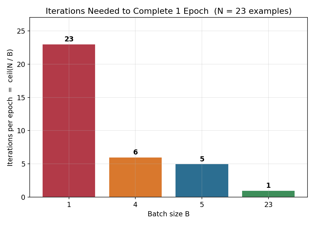
Bar chart showing iterations per epoch for batch sizes 1, 4, 5, and 23, given a dataset of 23 examples, with values 23, 6, 5, and 1 respectively
Notice batch size needs iterations, not — that’s the ceiling function doing its job: five full batches of 4 ( examples) plus one leftover batch of just 3.
4.4 Geometric / Intuitive Interpretation
Go back to the descent-path pictures from the Gradient Descent notes: each dot along that path was one iteration — one application of the update rule. An epoch doesn’t add a new kind of dot; it’s simply a checkpoint you reach after enough dots have been placed to guarantee the model has now looked at every training example exactly once. A smaller batch size means more, closer-together dots per epoch (and a noisier path, as you saw with the SGD path in that diagram); a larger batch size means fewer, more widely spaced dots per epoch (and a smoother path) — but either way, it still takes exactly epochs to show the model the dataset times.
5. Types / Variants
The Gradient Descent notes already introduced batch, mini-batch, and stochastic gradient descent based on how much data is used per step. Here’s the same three choices, but now viewed through the epoch/iteration lens — i.e., how many iterations each choice actually produces per epoch.
| Type | Analogy | Batch size | Iterations per epoch | Update frequency | Noise per iteration |
|---|---|---|---|---|---|
| Full-batch training | Reading the entire textbook cover-to-cover before updating your understanding once | Very infrequent | None (uses all data every time) | ||
| Mini-batch training | Reading one chapter at a time, updating your understanding after each chapter | Moderate | Moderate | ||
| Stochastic (online) training | Updating your understanding after every single sentence | Extremely frequent | High |
With full-batch training, one epoch is one iteration — the two concepts collapse into the same event, exactly like they did in the very first learning machines described in Section 2. As soon as drops below , an epoch starts containing multiple iterations, and that’s precisely the moment “epoch” and “iteration” needed to become two separate words.
6. Limitations, Failure Modes, and Trade-offs
Too few epochs → underfitting. If you stop training after just epoch 1 (only 5 iterations in our worked example), the model has barely nudged its parameters away from their starting guess — much like reading a chapter once and expecting to have mastered it. The loss is usually still high, and the model hasn’t had enough repeated exposure to the data to learn its underlying patterns.
Too many epochs → overfitting. Push training too far in the other direction, and something more subtle goes wrong: the training loss keeps dropping, but performance on data the model hasn’t seen (measured with a held-out validation set) starts getting worse. The model isn’t learning general patterns anymore — it’s starting to memorize quirks specific to the training examples.
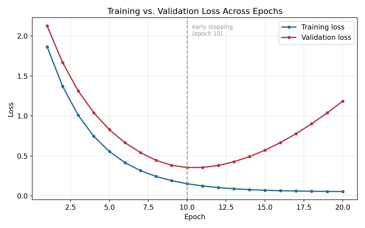
Line chart of training loss steadily decreasing across 20 epochs, and validation loss decreasing until around epoch 10 then increasing again, with a dashed line marking the early stopping point at epoch 10
In this example, training loss keeps falling smoothly all the way to epoch 20, but validation loss bottoms out around epoch 10 and then climbs back up — a textbook sign of overfitting. Training past that point isn’t just wasted computation; it actively makes the model worse at its actual job of handling new, unseen data.
How this is addressed: early stopping — monitor the validation loss after every epoch, and stop training (or keep a saved copy of the best-so-far model) once it stops improving for a set number of epochs, rather than training for some arbitrarily fixed number. This directly uses the epoch-by-epoch structure discussed in this document: the check happens once per epoch, not once per iteration, because a single iteration’s loss is far too noisy to base a stopping decision on (see the diagram below).
A practical gotcha worth flagging: the word “iteration” is not used consistently across libraries, papers, and codebases — some older texts and tools use “iteration” to mean what we’ve called an epoch here (one full data pass), while others (and the convention used in this document, matching most modern deep learning frameworks) use it to mean one single batch update. Always check which one a given tool or paper means before comparing hyperparameters like “number of iterations” across sources.
Batch size also affects how noisy your iteration-level loss looks, independent of epochs or overfitting:
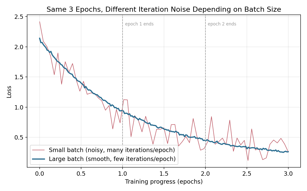
Line chart comparing loss per iteration for a small batch size, which is very noisy iteration-to-iteration, versus a large batch size, which is smooth, both following the same overall downward trend across 3 epochs marked by dashed vertical lines
This is the same noise-vs-smoothness trade-off from the Gradient Descent notes’ batch/mini-batch/SGD comparison, now shown as a loss curve over iterations rather than a path on a contour plot — same underlying phenomenon, different view of it.
7. Where This Connects to What You Already Know
Everything in this document is really just a more precise description of things already sitting inside the Gradient Descent notes:
- The update rule from those notes is exactly what happens once per iteration here — nothing new was added mathematically, we’ve just given a name to “one execution of that line.”
- The Batch GD / Mini-batch GD / SGD comparison from that document is the same comparison as Section 5 here, just now quantified in terms of how many iterations each choice produces per epoch.
- The worked linear regression example from those notes — where one gradient descent step dropped the loss from 15 to 0.234 — was, in this document’s language, iteration 1 of what would become epoch 1, if we kept looping through the (admittedly tiny, 3-example) dataset.
- Momentum and adaptive optimizers (Adam, RMSProp, mentioned in the earlier notes) keep internal memory that persists across iterations and epochs — the epoch/iteration structure here is exactly the clock that memory ticks along with.
8. Quick Recap Table
| Concept | Meaning |
|---|---|
| Dataset size | Total number of training examples |
| Batch size | Number of examples used in one iteration |
| Iteration / step | One single parameter update, using one batch |
| Epoch | One complete pass through the entire dataset |
| Iterations per epoch | — how many batches (iterations) it takes to cover the dataset once |
| Total iterations | — iterations per epoch, times the number of epochs |
| Full-batch training | ; one epoch = one iteration |
| Stochastic (online) training | ; most iterations per epoch, noisiest updates |
| Underfitting | Stopping training too early — too few epochs to learn the underlying patterns |
| Overfitting | Training too long — the model starts memorizing training data instead of generalizing |
| Early stopping | Monitoring validation loss per epoch and halting once it stops improving |
Key Takeaway
An epoch is one full lap through your entire dataset, and an iteration is one single step of gradient descent taken along the way — the same update rule you already know, just applied once per batch instead of once per dataset. How many iterations fit inside one epoch is entirely decided by your batch size, and how many epochs you run decides whether your model has learned enough (too few) or has started memorizing instead of generalizing (too many). Keeping these two clocks — iterations ticking fast within an epoch, epochs ticking slowly across the whole run — clearly separated in your head is what makes reading training logs, tuning hyperparameters, and diagnosing overfitting make sense.