Polynomial Regression
1. Introduction
Imagine you’re a car engineer studying how a car’s speed affects its fuel efficiency. You collect data from 40 cars driving at different speeds and plot fuel efficiency against speed. What do you see?
At low speeds, efficiency is poor (the engine works inefficiently at idle-like speeds). As speed increases, efficiency climbs, peaks somewhere around a moderate speed — and then drops again at high speeds because of air resistance and engine strain. The relationship isn’t a straight line at all — it’s a curve, roughly shaped like an upside-down bowl.
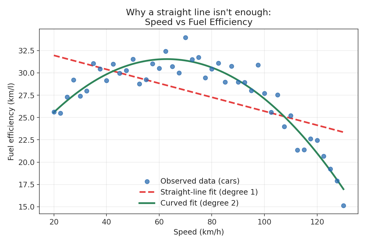
Why a straight line isn’t enough: speed vs fuel efficiency
Now, if you tried to fit a plain straight line through this data (like ordinary linear regression does), you’d get a poor, misleading result — the red dashed line above barely follows the real trend. But the green curve — which bends to match the data — tells the true story.
That bend is exactly what polynomial regression gives you. It’s a way of teaching a regression model to draw curves instead of being stuck with straight lines, simply by adding new “helper” features like , , and so on, built from your original input.
Formal definition: Polynomial regression is a form of regression analysis in which the relationship between the independent variable and the dependent variable is modeled as an -th degree polynomial in . It still belongs to the broader supervised learning family in machine learning — specifically, it’s a regression task (predicting a continuous number), the same category as linear regression, just with more flexibility to bend and curve.
Think of ordinary linear regression as a rigid wooden ruler you’re trying to lay across scattered dots — it can tilt, but it can never bend. Polynomial regression swaps that ruler for a flexible wire, letting the fit curve gently (or wildly, if you’re not careful) to match the true shape of the data.
2. History
The story of polynomial regression begins not with machine learning, but with astronomy in the early 1800s.
Scientists tracking the orbits of comets and planets had messy, noisy observational data, and they needed a systematic way to fit the best possible curve through it. In 1805, the French mathematician Adrien-Marie Legendre published the method of least squares — a technique for finding the curve that minimizes the total squared error between predictions and observations. Just a few years later, Carl Friedrich Gauss claimed he had actually been using the same method since 1795, sparking one of the most famous priority disputes in the history of mathematics. Regardless of who came first, least squares became the mathematical backbone that polynomial regression still relies on today.
At first, this method was mostly used to fit straight lines. But mathematicians quickly realized something elegant: if you simply treat , , and higher powers of as additional inputs, the same least-squares machinery used for straight lines could just as easily fit curves. Nothing new had to be invented — it was a clever reuse of the same idea, extended one small step further.
Later in the 19th century, the term “regression” itself was coined by Francis Galton, who studied how the heights of children related to the heights of their parents (his famous “regression toward the mean”). His student Karl Pearson helped formalize correlation and regression mathematically, cementing the statistical foundation that polynomial regression stands on.
For much of the early 20th century, fitting anything beyond a quadratic (degree 2) curve was tedious — it meant solving systems of equations by hand. Everything changed with the arrival of computers in the mid-1900s. Suddenly, statisticians and scientists could fit degree-10, degree-20, or even higher polynomials in seconds. This power came with a hidden trap: analysts began noticing that very high-degree polynomials fit their training data almost perfectly, yet made wild, nonsensical predictions on new data. This failure mode (which you’ll see demonstrated later in this document) pushed statisticians to invent regularization. In 1970, Arthur Hoerl and Robert Kennard introduced ridge regression, a technique that gently discourages a model’s coefficients from growing too large — effectively taming the wild curves of high-degree polynomials.
This idea of “add flexibility, but control it” didn’t stop there — it became a core theme that carries all the way into modern deep learning, where neural networks use similar regularization tricks (like weight decay) to prevent overly flexible models from memorizing noise instead of learning real patterns.
3. Core Concepts
3.1 Where Polynomial Regression Sits in Machine Learning
Before diving into the mechanics, it helps to place polynomial regression on the map of machine learning types:
| Machine Learning Type | What it does | Where Polynomial Regression Fits |
|---|---|---|
| Supervised Learning | Learns from labeled input-output pairs | ✅ Polynomial regression is supervised — it learns from pairs |
| Unsupervised Learning | Finds patterns in unlabeled data | ❌ Not applicable here |
| Reinforcement Learning | Learns via rewards from actions | ❌ Not applicable here |
| — Regression (subtype) | Predicts a continuous number | ✅ This is exactly what polynomial regression does |
| — Classification (subtype) | Predicts a category/class | ❌ Not this |
So polynomial regression is simply a more flexible cousin of linear regression, living in the “supervised regression” branch of machine learning.
3.2 From a Straight Line to a Curve
Ordinary linear regression predicts using a straight-line equation:
This works beautifully when your data genuinely follows a straight-line trend. But real-world relationships (fuel efficiency vs. speed, plant growth over time, projectile motion, etc.) often curve. Instead of abandoning the linear regression toolbox entirely, polynomial regression makes a clever move: it keeps the same least-squares fitting machinery, but feeds it new, engineered features — — in addition to itself.
This is the single biggest idea to understand: polynomial regression is still linear regression — just linear in the coefficients, not in . The curve you see is really a straight-line relationship in a higher-dimensional feature space.
3.3 Building Up the Model, Degree by Degree
| Degree () | Equation | Shape | Typical Use Case |
|---|---|---|---|
| 0 | Flat horizontal line | Predicting a constant average | |
| 1 | Straight line | Simple linear trends (e.g., height vs. age in early growth) | |
| 2 | Single bend (parabola) | Peak/valley trends (e.g., speed vs. fuel efficiency) | |
| 3 | S-shaped curve, up to 2 bends | More complex trends (e.g., population growth with a plateau) | |
| (high) | Up to bends | Rare — usually a sign of overfitting risk |
Each row builds on the previous one by adding just one more term — the model doesn’t change its fundamental strategy, it just gets access to one more “shape-bending” tool.
3.4 Connecting to Neurons and Perceptrons
Here’s where this connects to structures you may already be familiar with. A biological neuron (and its simplified computational cousin, the perceptron) works by taking several inputs, multiplying each by a weight, summing them up, adding a bias, and then passing the result through an activation function:
Look closely — that weighted sum has exactly the same mathematical shape as our polynomial regression equation ! In both cases, we’re computing a linear combination of features and adding a bias term.
The key difference is where the nonlinearity comes from:
- In polynomial regression, you manually decide the nonlinear features (, , …) before the linear combination happens.
- In a perceptron/neuron, the nonlinearity comes after the linear combination, via the activation function (like a step function or sigmoid).
- In deep learning (stacks of neurons in layers), the network automatically learns what nonlinear features are useful — instead of a human guessing “maybe I need and ,” the hidden layers discover far richer, data-driven transformations on their own.
In other words: polynomial regression is a hand-engineered, shallow way of adding curvature to a model — deep learning automates and generalizes that same idea.
4. The Math Behind Polynomial Regression
4.1 Starting Point: Simple Linear Regression
We begin with the familiar linear regression formula:
where is the intercept, is the slope, and is the error term (the gap between prediction and reality). This works only when the true relationship is (approximately) a straight line.
4.2 Why We Need More Terms
If the true relationship curves — like our fuel efficiency example — a single slope cannot capture a bend. A straight line has a constant rate of change; a curve does not. So we need a term whose contribution changes as changes. Adding does exactly that: its rate of change itself depends on , letting the model bend.
4.3 Building the Polynomial Formula, Step by Step
Step 1 — Add a quadratic term to allow one bend:
Step 2 — Add a cubic term to allow an inflection point (an S-curve):
Step 3 — Generalize to any degree :
Why this makes sense in plain words: each new power of acts like a new “shape adjustment knob.” controls the overall tilt, controls how much it bows into a single curve, lets it wiggle with an S-shape, and so on. The higher the degree, the more knobs you have to sculpt the curve — but as we’ll see in the Limitations section, too many knobs becomes dangerous.
4.4 Why It’s Still Called “Linear” Regression
This confuses many learners at first: the curve is clearly nonlinear in , so why call it “linear regression”? The answer is that linearity here refers to the coefficients ( values), not to . If you define new variables:
then the equation becomes:
which is exactly the form of ordinary multiple linear regression! We’ve simply relabeled our features. This means we can reuse all the standard linear regression machinery — including the Design Matrix and Normal Equation — without inventing anything new.
4.5 The Design Matrix (Vandermonde Matrix)
For data points, we organize the powers of into a matrix:
Each row is one data point; each column is one power of . This special structure is called a Vandermonde matrix.
4.6 The Cost Function (What “Best Fit” Means)
To find the best coefficients , we minimize the Mean Squared Error (MSE) between predictions and actual values :
Why squared error, in plain words: squaring makes all errors positive (so overestimates and underestimates don’t cancel out) and it punishes large errors much more than small ones — pushing the model to avoid big mistakes.
4.7 Solving for the Best Coefficients — The Normal Equation
Since this is still a linear regression problem in disguise, the optimal coefficients have a closed-form solution:
Intuition: this formula finds the exact point where the cost function is at its minimum — geometrically, the bottom of a smooth, bowl-shaped error surface. (In practice, for large or ill-conditioned , this is often solved with gradient descent or numerically stable decomposition methods instead of directly inverting the matrix.)
4.8 Geometric Interpretation
Here’s the elegant part: in the original 1-dimensional space of , the fitted model looks like a bending curve. But in the expanded feature space of , that same model is a perfectly flat hyperplane. Polynomial regression doesn’t actually know how to “curve” — it only knows how to draw straight hyperplanes. The curvature we see is simply the shadow that flat hyperplane casts back down into the original, lower-dimensional space of and .
5. Types / Variants of Polynomial Regression
Not all polynomial regression is created equal. Here are the main variants you’ll encounter:
- Simple Polynomial Regression — one input variable raised to increasing powers. Analogy: sculpting a single strand of wire into a curve.
- Multivariate Polynomial Regression — multiple input variables, each raised to powers, plus interaction terms (like ). Analogy: sculpting a flexible sheet of clay in more than one direction at once, where bending it along one axis also affects the other.
- Orthogonal Polynomial Regression — instead of using plain powers (), it uses specially designed polynomial “basis functions” (like Chebyshev or Legendre polynomials) that don’t overlap or correlate with each other. Analogy: instead of stacking transparent colored sheets that blur together (regular powers, which are highly correlated), you use sheets with perfectly distinct, non-overlapping colors — much easier to separate their individual effects.
- Regularized Polynomial Regression (Ridge/Lasso Polynomial) — adds a penalty term that discourages coefficients from growing too large, taming wild curves. Analogy: attaching light springs to your flexible wire so it resists bending too sharply, keeping it smooth even when tempted to chase every noisy data point.
Comparison Table
| Variant | Inputs Used | Main Strength | Main Weakness | Best For |
|---|---|---|---|---|
| Simple Polynomial Regression | One variable () | Easy to understand and visualize | Can’t model multi-feature interactions | Single-feature curved trends |
| Multivariate Polynomial Regression | Multiple variables + interactions | Captures combined effects between features | Number of terms explodes quickly | Complex, multi-factor systems |
| Orthogonal Polynomial Regression | Transformed basis functions | Numerically stable, less correlated terms | Slightly harder to interpret coefficients directly | High-degree fits needing stability |
| Regularized Polynomial Regression | Any of the above + penalty | Controls overfitting automatically | Needs tuning of the penalty strength | Noisy data, high-degree models |
6. Limitations, Failure Cases, and How They Were Addressed
6.1 Overfitting — Too Much Flexibility
The most notorious limitation of polynomial regression is overfitting: a high-degree polynomial can pass through (or very close to) every single training point, but it does so by wiggling wildly between them — making terrible predictions on new data.
Worked example: Using the exact same dataset, look what happens as we increase the degree:
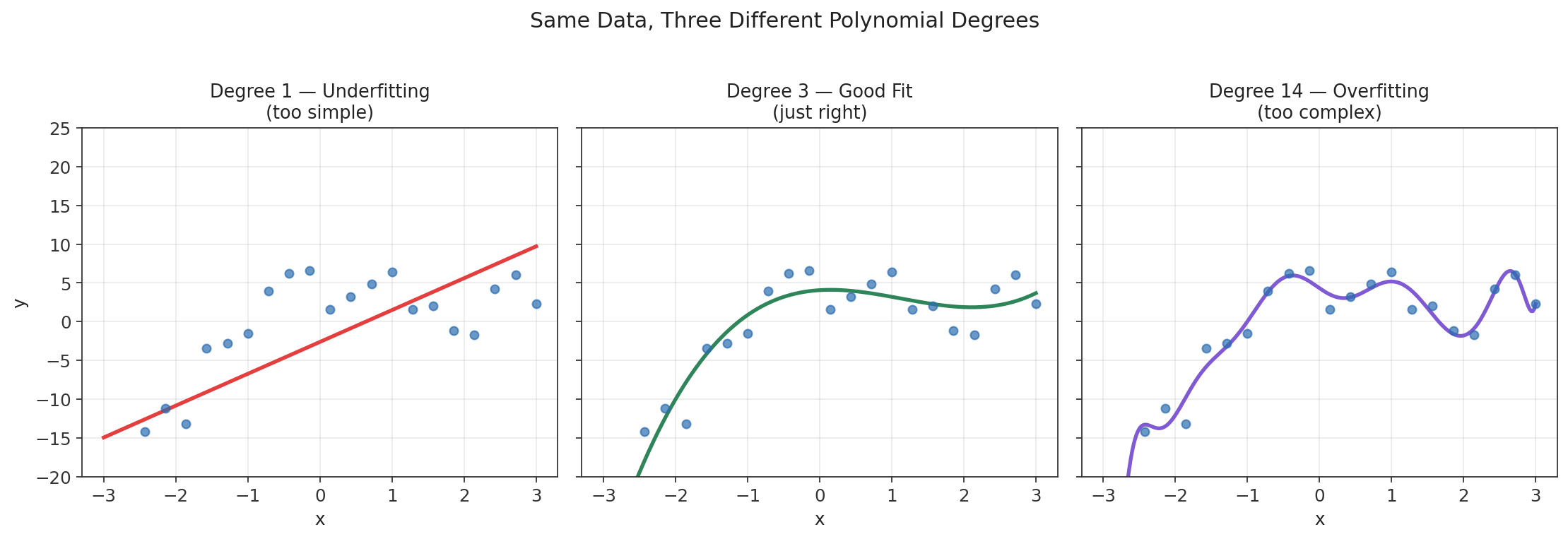
Underfitting vs good fit vs overfitting across three polynomial degrees
- Degree 1 (left): the line is too rigid — it misses the actual bend in the data entirely. This is underfitting (high bias).
- Degree 3 (middle): the curve smoothly captures the real trend without chasing every noisy point. This is the sweet spot.
- Degree 14 (right): the curve contorts itself to touch nearly every data point, producing unnatural wiggles that don’t reflect any real pattern. This is overfitting (high variance).
This tradeoff can be visualized directly by plotting error against polynomial degree:
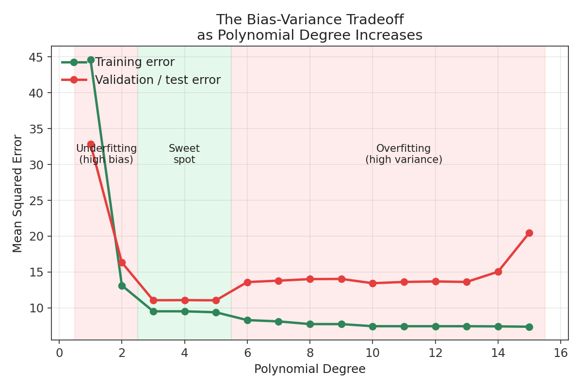
Bias-variance tradeoff as polynomial degree increases
Notice how training error keeps dropping as degree increases (the model memorizes the training data better and better), while validation error drops initially, hits a minimum, and then rises sharply — the classic signature of overfitting.
6.2 Runge’s Phenomenon — An Extreme Failure Case
A particularly dramatic version of this problem is called Runge’s Phenomenon, discovered by Carl Runge in 1901. Even with a mathematically “perfect” high-degree fit through evenly spaced points, the polynomial can swing wildly near the edges of the data range:
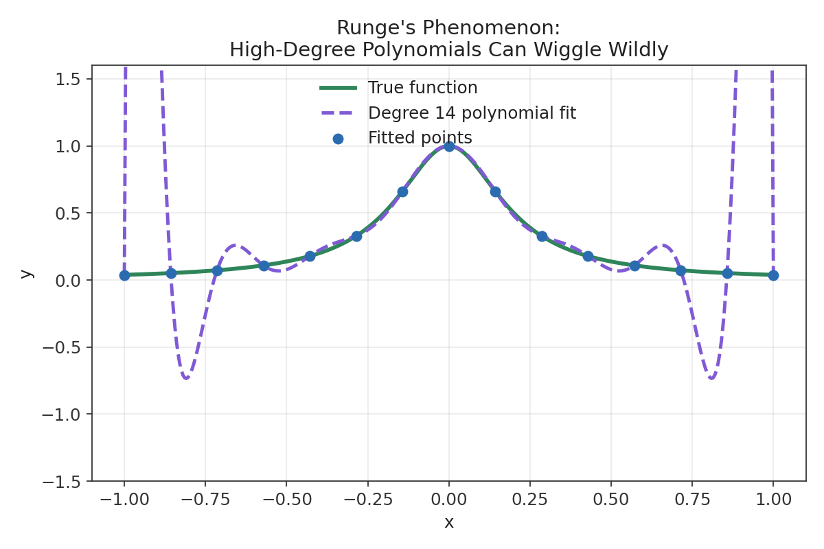
Runge’s phenomenon: high-degree polynomial fit oscillating near the edges
Here, a degree-14 polynomial passes exactly through all 15 sample points from a smooth true function — yet between and beyond those points (especially near the edges), it oscillates dramatically, deviating far from the true curve. This shows that “fitting every point perfectly” is not the same as “modeling the true relationship well.”
6.3 Extrapolation Danger
Polynomials behave especially badly outside the range of the training data. Because high-degree terms grow extremely fast, predicting even slightly beyond your observed values can produce wildly unrealistic results (like predicting negative fuel efficiency at very high speeds).
6.4 Multicollinearity
For higher degrees, the features become highly correlated with each other (they’re all just different powers of the same number), making the coefficient estimates unstable and difficult to interpret.
6.5 How These Limitations Were Addressed
- Regularization (Ridge/Lasso, from the History section) directly penalizes large coefficients, smoothing out the wild wiggles seen in overfitting and Runge’s phenomenon.
- Cross-validation is used to systematically choose the “just right” degree — comparing validation error across degrees (as in the bias-variance chart above) instead of guessing.
- Orthogonal polynomials reduce the multicollinearity problem by using non-overlapping basis functions.
- Splines / piecewise polynomials fit separate, low-degree polynomials to small chunks of the data and stitch them together smoothly, avoiding the need for one giant high-degree polynomial at all.
- Deep learning takes this evolution one step further: rather than a human manually choosing which powers of to add, neural networks learn their own nonlinear feature transformations directly from data, with regularization techniques (like weight decay and dropout) built in to prevent the same kind of overfitting seen here.
7. Quick Recap Table
| Concept | Meaning |
|---|---|
| Polynomial Regression | Regression that models as a polynomial (powers of ) instead of a straight line |
| Degree () | The highest power of used in the model; controls flexibility/curviness |
| Linear in Parameters | The model is still “linear regression” because it’s linear in the coefficients, not in |
| Design/Vandermonde Matrix | The matrix of raised to increasing powers, used to organize the data for fitting |
| Cost Function (MSE) | Measures how far predictions are from actual values; squared to penalize big errors |
| Normal Equation | Closed-form formula that directly solves for the best coefficients |
| Underfitting | Model too simple (low degree) — misses the real trend (high bias) |
| Overfitting | Model too complex (high degree) — memorizes noise instead of the trend (high variance) |
| Runge’s Phenomenon | Extreme oscillation of high-degree polynomials near the edges of the data range |
| Regularization (Ridge/Lasso) | Technique that penalizes large coefficients to prevent overfitting |
| Orthogonal Polynomials | Non-overlapping polynomial basis functions used for numerical stability |
| Connection to Neurons/Perceptrons | Both compute a weighted sum of features + bias — polynomial regression pre-engineers the nonlinearity, while neurons apply it via activation functions |
| Connection to Deep Learning | Deep learning automates the “feature engineering” that polynomial regression does manually, learning nonlinear patterns directly from data |
8. Key Takeaway
Polynomial regression is what you get when you give ordinary linear regression the ability to bend — by feeding it engineered features like and instead of inventing a new algorithm entirely. It remains “linear” in its coefficients, solvable with the same least-squares math that’s been used since Legendre and Gauss, but its curvy flexibility is a double-edged sword: too little degree underfits reality, while too much degree memorizes noise and collapses into wild, unstable predictions (as Runge’s Phenomenon dramatically shows). The techniques invented to tame this — regularization, cross-validation, and smarter basis functions — became foundational ideas that echo forward into modern deep learning, where neural networks learn their own curves instead of relying on a human to hand-pick which powers of to use.